Carrying Out a Two-Sample t Test — AP® Statistics Notes

This is the last procedure of Unit 4, and it reuses everything before it: the standard error of a difference from the two-sample interval, the logic of a significance test from the one-sample t test, and the setup from the previous topic. What is new is one formula, the two-sample t statistic, and the habit of choosing among all the procedures you now know.

The two-sample t statistic

Assume $H_0$ is true: the true means are equal, so $\mu_1 - \mu_2 = 0$ . Then the difference in sample means, $\bar{x}_1 - \bar{x}_2$ , varies around 0 with standard error $\sqrt{\frac{s_1^2}{n_1} + \frac{s_2^2}{n_2}}$ . Measure the observed difference in standard errors:

$t = \frac{(\bar{x}_1 - \bar{x}_2) - 0}{\sqrt{\frac{s_1^2}{n_1} + \frac{s_2^2}{n_2}}}.$

This is the two-sample t statistic. Its p-value comes from a t distribution with the technology (Welch) degrees of freedom, or with the conservative df, the smaller of $n_1 - 1$ and $n_2 - 1$ . The conservative choice gives a slightly larger p-value; both are accepted.

The t distribution with 40.0 degrees of freedom, centered at 0. A dashed line marks the observed two-sample t statistic -2.31, and the small area to its left is shaded: the one-sided p-value, 0.0132. — **Figure 1.** The null model for the caffeine test and the shaded left-tail p-value. LevlPrep original diagram.

A complete test

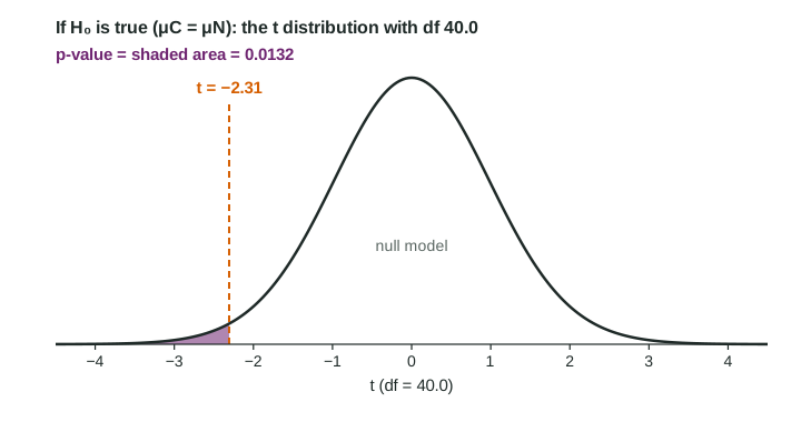
Worked example 1. Forty-two volunteers were randomly assigned to a caffeinated drink (C, $n = 20$ ) or a caffeine-free look-alike (N, $n = 22$ ), then did a reaction-time task (invented data). Caffeine: $\bar{x} = 241$ ms, $s = 28$ ; no caffeine: $\bar{x} = 262$ ms, $s = 31$ . Dotplots of both groups show no strong skew or outliers. Is there convincing evidence at $\alpha = 0.05$ that caffeine lowers mean reaction time?

State. $H_0: \mu_C - \mu_N = 0$ , $H_a: \mu_C - \mu_N < 0$ , where $\mu_C$ and $\mu_N$ are the true mean reaction times with and without caffeine for adults like these volunteers.

Plan. Two-sample t test. Random: random assignment to the two drinks. 10%: not needed for an experiment. Normal/large sample: both groups are under 30, but neither dotplot shows strong skew or outliers.

Do. $t$ $= \frac{241 - 262}{\sqrt{\frac{28^2}{20} + \frac{31^2}{22}}}$ $= \frac{-21}{\sqrt{39.2 + 43.68}}$ $= \frac{-21}{9.10}$ $= -2.31$ . Technology df 40.0; the alternative is "less than", so $p$ $= P(t < -2.31)$ $= 0.0132$ . (Conservative df 19: $p = 0.0163$ .)

Conclude. Because the p-value of 0.0132 is less than 0.05, we reject the null hypothesis. There is convincing evidence that the true mean reaction time with caffeine is less than without caffeine, for adults like these.

Scope. The drinks were randomly assigned, so the faster reactions can be credited to caffeine. The volunteers were not a random sample, so the result applies to adults like them.

Worked example 2 (two-sided, fail to reject). Independent random samples of adults in two large counties: county 1, $n = 45$ , $\bar{x} = 4.6$ hours of exercise last week, $s = 2.9$ ; county 2, $n = 50$ , $\bar{x} = 3.9$ , $s = 3.3$ . Test $H_0: \mu_1 - \mu_2 = 0$ against $H_a: \mu_1 - \mu_2 \ne 0$ at $\alpha = 0.05$ .

Conditions: independent random samples; each is less than 10% of its county's adults; both $n \ge 30$ .

$t$ $= \frac{4.6 - 3.9}{\sqrt{\frac{2.9^2}{45} + \frac{3.3^2}{50}}}$ $= \frac{0.7}{0.636}$ $= 1.10$ , technology df 93.0, two-sided $p = 2P(t > 1.10) = 0.274$ .

Because the p-value of 0.274 is greater than 0.05, we fail to reject the null hypothesis. There is not convincing evidence that the true mean weekly exercise hours of adults differ between the two counties.

The p-value in context: Assuming there is no difference in the true mean weekly exercise hours of the two counties, there is a 0.274 probability of getting a difference in sample means of 0.7 hours or more in either direction by chance, with random samples of 45 and 50 adults.

Having failed to reject, the department might have made a Type II error: the true means could differ by an amount these samples could not detect. A rejection, like the caffeine result, risks a Type I error instead.

Choosing the inference procedure

Unit 3 and Unit 4 together give you a small family of procedures. Three questions pick the right one.

Question	If	Then
1. What is the response?	categorical (yes or no)	proportions: z procedures
	categorical with several categories, in a two-way table	chi-square test for homogeneity or independence (Unit 3)
	quantitative (a measurement)	means: t procedures
2. How many groups, and how linked?	one sample, or paired data	one-sample t (paired: on the differences)
	two independent groups	two-sample t
3. What is asked?	"estimate", "how much"	confidence interval
	"is there convincing evidence", a claim	significance test

For example, a teacher who measures each student's score before and after a review game has a quantitative response and paired data: a paired t test on the differences. A researcher comparing the proportion of adults who exercise at least 3 hours a week in two counties has a categorical response and two groups: a two-sample z test for proportions.

Common slips

Adding standard errors instead of variances in the denominator.
Switching the order of subtraction between the hypotheses, the statistic and the conclusion.
Doubling (or not doubling) the tail area: one tail for $<$ or $>$ , two for $\ne$ .
Concluding "the means are equal" after failing to reject.
Claiming cause and effect from two random samples, or generalizing to a population from volunteers.