Interval for a Proportion — AP® Statistics Notes

A point estimate such as $\hat{p} = 0.62$ is our best single guess, but it is almost never exactly right. A confidence interval gives a range of values instead, built so that the method captures the true proportion a known percent of the time. This topic is about building one correctly; the next topic is about what it lets you say.

The idea: go out a fixed distance on each side

From the last topic, when the conditions hold, $\hat{p}$ is approximately normal with mean $p$ and standard deviation $\sqrt{p(1 - p)/n}$ . In 95% of random samples, $\hat{p}$ lands within 1.96 standard deviations of $p$ . Turn that sentence around: in 95% of samples, $p$ is within 1.96 standard deviations of $\hat{p}$ . So if we go 1.96 standard deviations out on each side of whatever $\hat{p}$ we get, 95% of the intervals we build that way will reach across $p$ .

Top: the normal sampling distribution of the sample proportion, centered at the unknown true proportion p, with the middle 95% shaded between p minus 1.96 standard deviations and p plus 1.96 standard deviations. Below it, three sample proportions are drawn with their intervals, each the sample proportion plus or minus 1.96 standard deviations. The two sample proportions that land inside the shaded middle 95% give intervals that reach across p; the one that lands in the tail gives an interval that misses p. — **Figure 1.** Sample proportions that land in the middle 95% of the sampling distribution give intervals that capture p; the ones in the tails give intervals that miss. LevlPrep original diagram.

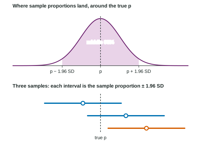
Every confidence interval in this course has the same shape, which is on the reference sheet:

statistic ± (critical value)(standard error of the statistic)

For one proportion that is

$\hat{p} \pm z^*\sqrt{\frac{\hat{p}(1 - \hat{p})}{n}}$

The three pieces

The point estimate $\hat{p}$ is the center of the interval.
The standard error, $\text{SE}$ $= \sqrt{\frac{\hat{p}(1 - \hat{p})}{n}}$ . The true standard deviation needs $p$ , which we do not know, so we substitute $\hat{p}$ . A standard deviation estimated from the data is called a standard error.
The critical value $z^*$ comes from the confidence level $C$ . It is the value with an area of $C$ between $-z^*$ and $z^*$ under the standard normal curve, so each tail holds $\frac{1 - C}{2}$ .

The product $z^* \cdot \text{SE}$ is the margin of error, $\text{ME}$ : how far the interval reaches on each side of $\hat{p}$ .

Confidence level	Area in each tail	Area below $z^*$	$z^*$
90%	0.05	0.95	1.645
95%	0.025	0.975	1.960
98%	0.01	0.99	2.326
99%	0.005	0.995	2.576

Find $z^*$ with an inverse normal command using the area below it, or from the bottom row of Table B. A common slip is to use 0.90 as the area for a 90% interval: that leaves all 10% in one tail.

Conditions for inference

Check three conditions, in words and with numbers, before you calculate.

Random: the data come from a random sample (or a randomized experiment). Quote the problem: "a random sample of 400 students."
10%: when sampling without replacement, $n$ is at most 10% of the population: "400 is less than 10% of the 28,000 students."
Large counts: at least 10 successes and 10 failures in the sample: $n\hat{p} \ge 10$ and $n(1 - \hat{p}) \ge 10$ . For an interval we use the sample's counts, because $p$ is unknown.

The procedure's full name is the one-sample z interval for a proportion (some books say one-proportion z interval). Name it on the exam; "z interval" alone is incomplete.

Worked example. A random sample of 400 of a university's 28,000 students finds that 248 regularly skip breakfast. Construct a 95% confidence interval for the proportion of all students at the university who regularly skip breakfast.

Procedure. One-sample z interval for a proportion, where $p$ is the true proportion of all students at the university who regularly skip breakfast.

Conditions. Random: a random sample of 400 students. 10%: 400 is less than 10% of 28,000 (2,800). Large counts: 248 skip and 152 do not, both at least 10.

Calculate. $\hat{p} = \frac{248}{400} = 0.62$ . $\text{SE}$ $= \sqrt{\frac{0.62(0.38)}{400}}$ $= 0.0243$ . For 95%, $z^* = 1.96$ , so $\text{ME}$ $= 1.96(0.0243)$ $= 0.0476$ .

$0.62 \pm 1.96\sqrt{\frac{0.62(0.38)}{400}} = 0.62 \pm 0.048$

Answer. The interval runs from 0.572 to 0.668. Technology (a one-proportion z interval) gives the same. Interpreted: we are 95% confident that the interval from 0.572 to 0.668 captures the true proportion of all students at the university who regularly skip breakfast.

Type an interval as "from 0.572 to 0.668" or "(0.572, 0.668)". Never "0.572-0.668", which reads as a subtraction.

What changes the margin of error

Sample size: $n$ sits under a square root in the denominator. Four times the sample size halves the margin of error.
Confidence level: more confidence needs a larger $z^*$ , so the interval gets longer. A 99% interval reaches farther than a 95% interval from the same data.
Population size: it does not appear, as long as the 10% condition holds.

To plan a sample size, solve $z^*\sqrt{\frac{\hat{p}(1 - \hat{p})}{n}} \le \text{ME}$ for $n$ : $n \ge \left(\frac{z^*}{\text{ME}}\right)^2\hat{p}(1 - \hat{p})$ . With no earlier estimate, use $\hat{p} = 0.5$ , which gives the largest $n$ and so is safe. Always round a sample size up.