Estimators — AP® Statistics Notes

Unit 3 is about using a sample to say something about a population. Before any formulas, we need a way to judge whether a sample's answer can be trusted. That judgment always comes from the same place: what the statistic does over many possible samples.

Estimators and point estimates

A parameter describes a whole population, and we usually cannot measure it. A statistic describes a sample, and we can. When we use a statistic to estimate a parameter, the statistic is called an estimator. The value it gives for one particular sample is a point estimate.

The sample proportion $\hat{p}$ estimates the population proportion $p$ .
The sample mean $\bar{x}$ estimates the population mean $\mu$ .
The sample standard deviation $s$ estimates the population standard deviation $\sigma$ .

If 124 of 400 randomly chosen voters support a new park, the point estimate of $p$ is $\hat{p} = \frac{124}{400} = 0.31$ . Another random sample of 400 would give a slightly different number. So a point estimate on its own tells you nothing about how far off it might be. To know that, look at the estimator's sampling distribution.

Bias: where the estimates center

Picture taking every possible sample of the same size with the same method and computing the statistic each time. Those values form the statistic's sampling distribution. An estimator is unbiased when the center (the mean) of its sampling distribution equals the parameter. It is biased when the center sits too high or too low.

Unbiased does not mean "right in every sample". It means "right on average". Single samples still land above or below the truth. They just do not lean one way.

Bias comes from the method. A random sample gives every member of the population a fair chance, so $\hat{p}$ from a random sample is an unbiased estimator of $p$ , and $\bar{x}$ is an unbiased estimator of $\mu$ . A method that favors some members (a convenience sample, a voluntary response poll) moves the center away from the parameter. Some statistics are biased even with random sampling. The sample maximum can never be larger than the population maximum, so it tends to come in too low as an estimate of it.

Variability: how spread out the estimates are

Variability is the spread of the sampling distribution. Low variability means the estimates from different samples are close to each other, so a typical estimate is close to its center.

For random samples, variability depends mostly on the sample size. Larger samples give less variable estimates. The spread shrinks with the square root of the sample size: four times as many observations cut the spread in half, not to a quarter. You will see the exact formula in the next topic. The size of the population barely matters, as long as it is much bigger than the sample.

Three probability histograms on the same scale from 0.1 to 0.8, each with a dashed line at the true proportion p = 0.40. Top: the sample proportion from random samples of 25 is centered at 0.40 and spread widely, from about 0.2 to 0.6: unbiased, high variability. Middle: the sample proportion from random samples of 100 is centered at 0.40 and about half as spread out: unbiased, low variability. Bottom: a biased method whose sample proportions center at 0.55 with low variability: biased, low variability. — **Figure 1.** Three estimators of p = 0.40. Random samples of 25 and of 100 are both centered on the truth; the larger sample is about half as spread out. A method that favors one group is centered at 0.55: precise, but precisely wrong. LevlPrep original diagram.

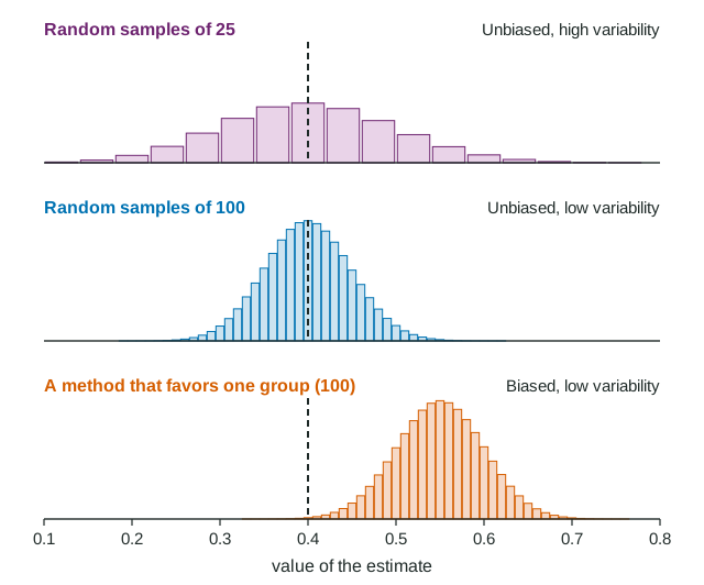
Bias and variability are separate problems

The figure shows three of the four combinations you need to tell apart; the table lists all four. Think of a target, with the parameter as the bullseye and each estimate as one arrow.

	Low variability	High variability
Unbiased	Arrows tightly grouped on the bullseye: the goal	Arrows scattered widely around the bullseye
Biased	Arrows tightly grouped, but off to one side	Arrows scattered, and centered off to one side

The fixes are different, too:

To reduce bias, change the method: select at random from the whole population.
To reduce variability, take a larger random sample.

A bigger sample does not fix a biased method. A website poll with 12,000 responses varies less from poll to poll than one with 1,200, but both are pulled the same way by who chooses to answer.

Worked example. In a shipment of 40,000 chargers, 8% are faulty ( $p = 0.08$ ). An inspector simulates four methods 1,000 times each. Method W (random samples of 50) gives sample proportions with mean 0.080 and standard deviation 0.038. Method X (random samples of 200): mean 0.080, standard deviation 0.019. Method Y (the first 200 packed on one shift): mean 0.052, standard deviation 0.016. Which method is best?

Bias. W and X center at 0.080, the parameter, so they are unbiased. Y centers at 0.052, below 0.08: it tends to underestimate the proportion of faulty chargers.

Variability. Y has the smallest spread (0.016), then X (0.019), then W (0.038). X uses $\frac{200}{50} = 4$ times as many chargers as W, and its spread is about $\frac{0.038}{\sqrt{4}} = 0.019$ .

Conclusion. Method X is best: it is unbiased and has low variability. Method Y is the least variable, but its estimates cluster around the wrong value, about 0.03 too low on average.

How the exam asks about this

Expect a table or plot of simulated values of two or more estimators, and questions such as "which is unbiased?", "which has the least variability?" or "which would you use, and why?". Answer with the center for bias and the spread for variability, and name both when you justify a choice. Always say it in context: "on average, this method underestimates the proportion of faulty chargers in the shipment."