Interval for Two Proportions — AP® Statistics Notes

In the last topic you learned how a difference of two sample proportions behaves when you know both true proportions. In real studies you know neither. You have two samples and want to estimate how far apart the populations are. A confidence interval for $p_1 - p_2$ does that job, and it is built exactly like the interval for one proportion: an estimate plus or minus a margin of error.

The parts of the interval

Every confidence interval in this course has the same structure:

statistic $\pm$ (critical value) $\times$ (standard error of the statistic)

For a difference of two proportions:

The statistic is the sample difference, $\hat{p}_1 - \hat{p}_2$ .
The critical value $z^*$ comes from the standard normal distribution: 1.645 for 90%, 1.96 for 95%, 2.576 for 99%.
The standard error is the standard deviation of $\hat{p}_1 - \hat{p}_2$ with each unknown $p$ replaced by its sample proportion.

Put together, the two-sample z interval for $p_1 - p_2$ is

$(\hat{p}_1 - \hat{p}_2) \pm z^* \sqrt{\frac{\hat{p}_1(1 - \hat{p}_1)}{n_1} + \frac{\hat{p}_2(1 - \hat{p}_2)}{n_2}}.$

Why the sample proportions in the standard error? Because we do not know $p_1$ and $p_2$ ; the whole point is to estimate them. The variances still add, just as in the last topic.

Conditions, in words, with numbers

Random: two independent random samples, or two groups formed by random assignment in an experiment. Say which, in the words of the problem.
10%: when sampling without replacement, each sample is less than 10% of its population. (In an experiment with no sampling, this check is not needed.)
Large counts: at least 10 successes and 10 failures in each sample: $n_1\hat{p}_1$ , $n_1(1 - \hat{p}_1)$ , $n_2\hat{p}_2$ and $n_2(1 - \hat{p}_2)$ are each at least 10. These are just the counts of yes and no answers in the data. Some books use 5; 10 is the common threshold.

Never check $n \ge 30$ for proportions. That rule belongs to means.

A full example

Number line showing a 95% confidence interval for the city minus suburbs difference in proportions: a dot at the estimate 0.08 and a bar from 0.006 to 0.154, a margin of error of 0.074 on each side, with a dashed line at 0 just left of the bar. — **Figure 1.** The interval as a picture: the estimate in the middle and a margin of error on each side. LevlPrep original diagram.

Worked example. A transit agency takes a random sample of 400 city residents and a separate random sample of 300 suburban residents. In the city, 248 say they would ride a new train line ( $\hat{p}_C = 0.62$ ); in the suburbs, 162 do ( $\hat{p}_S = 0.54$ ). Construct and interpret a 95% confidence interval for $p_C - p_S$ .

Name the procedure and the parameter. A two-sample z interval for $p_C - p_S$ , where $p_C$ is the true proportion of all city residents who would ride the line and $p_S$ is the true proportion of all suburban residents who would.

Conditions. Random: the problem says two separate random samples. 10%: 400 is less than 10% of city residents and 300 is less than 10% of suburban residents. Large counts: 248, 152, 162 and 138 are each at least 10.

Calculate. $\text{SE}$ $= \sqrt{\frac{0.62(0.38)}{400} + \frac{0.54(0.46)}{300}}$ $= \sqrt{0.000589 + 0.000828}$ $= 0.0376$ .

$(0.62 - 0.54)$ $\pm 1.96(0.0376)$ $= 0.08$ $\pm 0.074$ , which is from 0.006 to 0.154.

On a calculator this is a 2-proportion z interval; type the counts (248 of 400, 162 of 300) and the level.

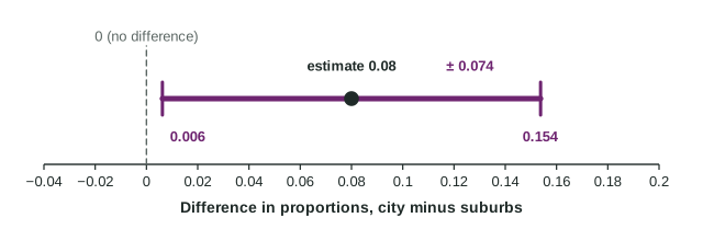
Interpret. We are 95% confident that the interval from 0.006 to 0.154 captures the true difference in the proportions of all city residents and all suburban residents who would ride the new train line (city minus suburbs).

The figure shows the same interval as a bar around the estimate. Notice the phrase "(city minus suburbs)". A difference has an order, and a reader needs to know which group came first. Subtract the other way and every sign flips: the interval for $p_S - p_C$ is from $-0.154$ to $-0.006$ .

What "95% confident" means

The 95% describes the method, not this one interval. If the agency took many pairs of random samples of these sizes and built a 95% interval from each, about 95% of those intervals would capture the true difference. Our interval either captures it or does not; we just do not know which.

Three readings to avoid:

"There is a 95% chance the true difference is in this interval." The true difference is a fixed number, not a random one.
"95% of city residents ..." The interval is about one number for the whole population, never about individuals.
Anything about the sample difference. We know it exactly: 0.08.

What changes the width

Change	Effect on the margin of error	Why
Higher confidence level	wider	$z^*$ is larger
Larger samples	narrower	each $n$ divides a variance; four times the $n$ halves the SE
Proportions near 0.5	wider	$\hat{p}(1 - \hat{p})$ is largest at 0.5

Experiments: random assignment

The same interval works for an experiment that randomly assigns subjects to two treatments. Random assignment takes the place of two random samples. It also changes what you can conclude: a difference between the groups can be blamed on the treatment, a cause-and-effect conclusion. If the subjects were volunteers rather than a random sample, generalize only to subjects like them.