Sampling Distribution of a Proportion

In the last topic you saw that a random sample's $\hat{p}$ is an unbiased estimator of $p$ , and that larger samples make it less variable. Now we pin that down with numbers: the exact center, the exact spread, and when the shape is close enough to normal to use a normal model. Every estimate and every judgment about a proportion later in this unit is built on this one sampling distribution.

Center, spread and shape

Take a random sample of size $n$ from a population in which a proportion $p$ have some characteristic (a "success"). The sample proportion is $\hat{p}$ $= \frac{\text{number of successes}}{n}$ . Over all possible samples, $\hat{p}$ has a sampling distribution with:

Center: $\mu_{\hat{p}} = p$ . This is the unbiasedness from the last topic, now as a formula.
Spread: the standard deviation of the sample proportion, $\sigma_{\hat{p}}$ $= \sqrt{\frac{p(1 - p)}{n}}$ . It is on the reference sheet.
Shape: approximately normal when the sample is large enough (the large counts condition, below).

Why this formula? One person's answer is a 1 (success) or a 0 (failure), and the standard deviation of such a 0-or-1 value is $\sqrt{p(1 - p)}$ . Averaging $n$ independent answers divides the spread by $\sqrt{n}$ . That is where the square root of $n$ comes from, and it is why 4 times the sample size halves the spread.

Notice that $p(1 - p)$ is largest when $p = 0.5$ ( $0.5 \times 0.5 = 0.25$ ). For a fixed sample size, proportions near one half are the hardest to pin down.

Two conditions, two different jobs

Students often mix these two up. They protect different parts of the model.

Condition	What to check	What it protects
10% condition	When sampling without replacement, $n$ is at most 10% of the population size	The standard deviation formula. Draws without replacement are then close to independent.
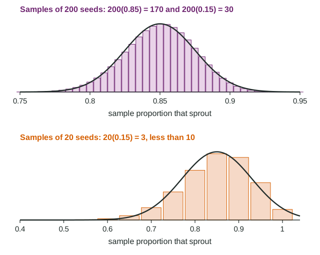
Large counts condition	$np \ge 10$ and $n(1 - p) \ge 10$ (some books use 5)	The normal shape. With at least 10 expected successes and 10 expected failures, the distribution is close to normal.

Random selection is a third requirement, and it is about bias: without it, the center of the sampling distribution is not $p$ , and no formula fixes that.

When large counts fails, the distribution is skewed. If $p$ is small, values pile up near 0 and stretch to the right; if $p$ is large, they pile up near 1 and stretch to the left. " $n \ge 30$ " is a rule of thumb for sample means and is never the check for proportions.

Two probability histograms of the sample proportion of seeds that sprout when the true proportion is p = 0.85. Top, samples of 200: the bars form a symmetric mound centered at 0.85 that matches the normal curve with mean 0.85 and standard deviation 0.025 drawn over it; large counts hold because 200(0.85) = 170 and 200(0.15) = 30 are both at least 10. Bottom, samples of 20: the bars are skewed left, piled up near 0.85 to 1 with a long tail toward lower values, and the normal curve does not fit; 20(0.15) = 3 is less than 10. — **Figure 1.** The exact sampling distribution of the proportion of seeds that sprout when p = 0.85. With 200 seeds the normal curve fits; with 20 seeds, 20(0.15) = 3 is less than 10 and the distribution is skewed left. LevlPrep original diagram.

Probabilities about a sample proportion

When both conditions hold, standardize $\hat{p}$ with its own mean and standard deviation and use the normal distribution:

$z = \frac{\hat{p} - p}{\sqrt{\frac{p(1 - p)}{n}}}$

Worked example. A seed company says 85% of its tomato seeds sprout. A store plants a random sample of 200 seeds from a shipment of 50,000. If the company is right, what is the probability that 80% or fewer of the 200 seeds sprout?

Conditions. 10%: 200 is less than 10% of 50,000 seeds (5,000). Large counts: $np$ $= 200(0.85)$ $= 170 \ge 10$ and $n(1 - p)$ $= 200(0.15)$ $= 30 \ge 10$ . So $\hat{p}$ is approximately normal.

Parameters. $\mu_{\hat{p}} = 0.85$ and $\sigma_{\hat{p}}$ $= \sqrt{\frac{0.85(0.15)}{200}}$ $= 0.0252$ .

Boundary and direction. We want $P(\hat{p} \le 0.80)$ , the area to the left of 0.80 under the normal curve with mean 0.85 and standard deviation 0.0252.

Calculate. $z$ $= \frac{0.80 - 0.85}{0.0252}$ $= -1.98$ , and $P(Z \le -1.98) = 0.024$ from Table A. Technology (a normal distribution with mean 0.85 and SD 0.0252, area below 0.80) gives 0.0239.

Tie it to the claim. If the company's 85% is correct, a sample this low would happen only about 2 times in 100 samples of 200 seeds. A result like that would make us doubt the company's figure.

Use the true $p$ in the standard deviation, not the sample value you are standardizing. In the worked example the standard deviation uses 0.85, never 0.80.

Count or proportion?

The number of successes, $X = n\hat{p}$ , is binomial with mean $np$ and standard deviation $\sqrt{np(1 - p)}$ . The proportion is that count divided by $n$ , so its mean is $p$ and its standard deviation is $\sqrt{p(1 - p)/n}$ . Read the question: "how many of the 200 seeds" is a count; "what proportion" or "what percent" is $\hat{p}$ . Mixing the two scales is a common slip.