Carrying Out a Chi-Square Test for…

In the last topic you set up a chi-square test: you chose independence or homogeneity, wrote the hypotheses, found the expected counts and checked the conditions. Now you finish the job. The statistic $\chi^2$ sums up how far the table is from the null hypothesis, a new family of distributions tells you how surprising that sum is, and the conclusion says what it means.

Components: cell by cell

For each cell, compare the observed count $O$ with the expected count $E$ and compute $\frac{(O - E)^2}{E}$ . This is the cell's chi-square component, its contribution to the total. Then add them all:

$\chi^2 = \sum \frac{(O - E)^2}{E}.$

A big component marks a cell where the data and $H_0$ disagree. Note that it is the gap relative to $E$ that matters. A gap of 10 where 30 were expected gives $\frac{100}{30} = 3.33$ ; the same gap where 60 were expected gives only $\frac{100}{60} = 1.67$ .

Degrees of freedom and the chi-square distribution

If $H_0$ is true and the conditions hold, the statistic follows (approximately) a chi-square distribution. There is one curve for each number of degrees of freedom; for a two-way table,

$\text{df} = (\text{rows} - 1)(\text{columns} - 1).$

Why that number? Once the row and column totals are fixed, you can fill in only $(r - 1)(c - 1)$ cells freely; the totals then force the rest. That count of free cells is the df.

Every chi-square curve starts at 0 (a sum of squares cannot be negative), is skewed right, and has its mean at the df. As the df grows, the curve spreads out and becomes more symmetric.

Only large values of $\chi^2$ are evidence against $H_0$ , so the p-value is always the area in the right tail, beyond the observed $\chi^2$ .

Right-skewed chi-square density curve with 2 degrees of freedom; a dashed line marks the observed statistic 8.21 and the thin shaded tail to its right is the p-value, 0.0165. — **Figure 1.** The chi-square curve with 2 degrees of freedom and the right tail beyond the observed statistic. LevlPrep original diagram.

Worked example. A random sample of 300 students at a large high school reports whether they keep a phone in the bedroom at night and their usual sleep. Test at $\alpha = 0.05$ whether the two variables are associated.

Phone in bedroom	Under 7 hours	7 to 8 hours	Over 8 hours	Total
Yes	70 (60)	90 (93.3)	40 (46.7)	200
No	20 (30)	50 (46.7)	30 (23.3)	100
Total	90	140	70	300

State. $H_0$ : there is no association between keeping a phone in the bedroom and usual sleep for students at the school. $H_a$ : there is an association.

Plan. A chi-square test for independence. Random: a random sample of 300 students. 10%: 300 is less than 10% of the students at a large school. Large counts: the expected counts in parentheses are each at least 5 (the smallest is 23.3).

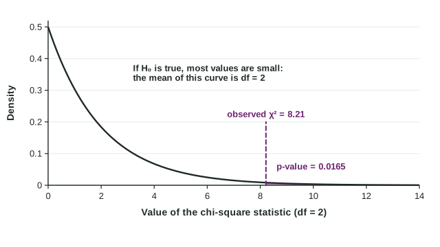
Do. $\chi^2$ $= \frac{(70 - 60)^2}{60}$ $+ \frac{(90 - 93.3)^2}{93.3}$ $+ \frac{(40 - 46.7)^2}{46.7}$ $+ \frac{(20 - 30)^2}{30}$ $+ \frac{(50 - 46.7)^2}{46.7}$ $+ \frac{(30 - 23.3)^2}{23.3}$

$= 1.67$ $+ 0.12$ $+ 0.95$ $+ 3.33$ $+ 0.24$ $+ 1.90$ $= 8.21$ , with $\text{df} = (2 - 1)(3 - 1) = 2$ .

The p-value is $P(\chi^2 \ge 8.21) = 0.0165$ , the right-tail area under the chi-square curve with 2 degrees of freedom. On a calculator, enter the observed counts as a matrix and run a chi-square test; it reports the same statistic, df and p-value and fills in the expected counts.

Conclude. Because the p-value of 0.0165 is less than $\alpha = 0.05$ , we reject $H_0$ . There is convincing evidence of an association between keeping a phone in the bedroom and usual hours of sleep for students at the school.

The figure shows how far out 8.21 sits: if there were no association, a value this large would happen less than 2% of the time.

Describing the association

A chi-square test says only that an association exists. To say what it looks like, use the table. The largest components here are the "no phone" row's under 7 hours (3.33) and over 8 hours (1.90) cells: students without a phone in the bedroom are less likely than expected to sleep under 7 hours and more likely to sleep over 8. In conditional percents, 35% of phone keepers sleep under 7 hours, against 20% of the others.

This was an observational study, so we cannot say phones cause less sleep; students who sleep less might keep their phones nearby for other reasons.

Reading Table C

Without technology, find the row for your df in Table C and see which critical values your $\chi^2$ falls between. For $\chi^2 = 9.8$ with 4 degrees of freedom, the row shows 9.49 (tail area 0.05) and 11.14 (tail area 0.025), so the p-value is between 0.025 and 0.05. Technology gives 0.044.

Wording to avoid

When the p-value is large, never say the variables "are independent" or the distributions "are the same". Say there is not convincing evidence of an association (or of a difference).
The alternative has no direction, so the conclusion does not either. Directions come from describing the table afterward.
For homogeneity, conclude about the distributions: "There is (is not) convincing evidence that the distribution of results differs between yoga and physical therapy for adults like these."