The setup of a test fixes the hypotheses and the standard of evidence. Now the data arrive, and we need one number that says how surprising they are if the null hypothesis is true. That number is the p-value. This topic is about computing it and, just as important, saying what it means.
The logic: assume , then ask how surprising the data are
A significance test argues like this. Suppose is true. Then the sampling distribution of is centered at , and we know its spread. If our sample proportion lands somewhere typical in that distribution, the data are consistent with . If it lands far out in a tail, in the direction points, then either something rare happened or is wrong. The rarer the result under , the stronger the evidence against it.
The test statistic
To measure "how far out", standardize. The reference sheet gives the general form of a standardized test statistic:
For one proportion, the statistic is , the parameter is its null value , and because we are assuming is true, the spread is computed with too:
Using inside the square root is the most common error on this calculation. An interval uses there because it has no null value; a test has one and must use it.
The p-value
The p-value is the probability, assuming is true, of getting a statistic at least as extreme as the one observed, in the direction of . Which area you find depends on the alternative:
| Alternative | p-value |
|---|---|
| area to the left of : | |
| area to the right of : | |
| both tails: |
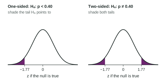
Worked example. A coffee chain says 40% of its customers order a pastry. A store manager suspects her store is lower. In a random sample of 300 of the store's orders, 105 include a pastry. Test against , where is the true proportion of all the store's orders that include a pastry. (Random, 10% and large counts, and , are met.)
Statistic. .
Test statistic.
p-value. says "less than", so find the left tail: (technology: a 1-proportion z test gives , p-value 0.0385; Table A gives 0.0384).
Interpretation. Assuming the true proportion of all the store's orders that include a pastry is 0.40, there is a 0.0385 probability of getting a sample proportion of 0.35 or less by chance in a random sample of 300 orders.
The interpretation has four parts: the condition ("assuming the true proportion is 0.40"), the probability, the statistic and direction ("0.35 or less"), and the sample ("a random sample of 300 orders"). For a two-sided test, say "at least as far from 0.40 as the observed value, in either direction".
A p-value from a simulation
You can also estimate a p-value without a formula. Simulate many samples in a world where is true, then count the simulated results at least as extreme as the real one. A player who claims to make 75% of her free throws makes 31 of 50 (). If 3 of 100 simulated sets of 50 shots by a 75% shooter come out at 0.62 or lower, the estimated p-value is . The dotplot of simulated results is centered at 0.75, not at 0.62, because it is built assuming .
What a p-value is not
- It is not the probability that is true. It is computed by assuming is true.
- A large p-value does not show that is true. It shows that the data are consistent with it.
- A small p-value is evidence against , not proof. Rare results do happen.
Smaller p-values come from results farther from in the direction of , and from larger samples, which shrink the standard deviation and so stretch the same difference into a larger . In the next topic you will compare the p-value with to reach a decision.