Two-Proportion Sampling Distribution — AP® Statistics Notes

Many of the most useful questions in statistics compare two groups. Do more teens than adults use a bike share? Does a new reminder text get more patients to show up than the old one? To answer them, you take a sample from each group and compare the two sample proportions. Before you can judge a comparison, you need to know how much a difference of two sample proportions moves around just by chance. That is what this topic is about.

A new statistic: the difference

Suppose a fraction $p_1$ of population 1 and a fraction $p_2$ of population 2 have some trait. Take a random sample of size $n_1$ from the first population and, separately, a random sample of size $n_2$ from the second. Each sample gives a sample proportion, $\hat{p}_1$ and $\hat{p}_2$ . The statistic we care about is their difference in sample proportions:

$\hat{p}_1 - \hat{p}_2.$

Like any statistic, it changes from sample to sample. Its sampling distribution has a center, a spread and a shape, and each one follows from what you already know about a single sample proportion.

Center: the difference of the true proportions

You know that $\hat{p}_1$ is centered at $p_1$ and $\hat{p}_2$ is centered at $p_2$ . So their difference is centered at the difference of the true proportions:

$\mu_{\hat{p}_1 - \hat{p}_2} = p_1 - p_2.$

This means $\hat{p}_1 - \hat{p}_2$ is an unbiased estimator of $p_1 - p_2$ . It is not always right, but it is not off in one direction on average.

Spread: the variances add

Here is the surprising part. Each sample proportion has its own chance error. When you subtract, those errors do not cancel. Sometimes $\hat{p}_1$ comes out high while $\hat{p}_2$ comes out low, and then the difference is far too big. The two errors pile up. So a difference of two independent statistics varies more than either one alone.

The rule is that the variances add (a variance is a standard deviation squared). For two independent samples:

$\sigma_{\hat{p}_1 - \hat{p}_2} = \sqrt{\frac{p_1(1 - p_1)}{n_1} + \frac{p_2(1 - p_2)}{n_2}}.$

Each term under the square root is the variance of one sample proportion. You add them first, then take one square root. Adding the two standard deviations, or subtracting anything, gives the wrong answer. This formula is on the reference sheet you get on the exam.

The formula needs independent samples: who ends up in one sample has nothing to do with who ends up in the other. Two separate random samples from two schools are independent. Husbands and their own wives are not, because each person in one sample is linked to a person in the other.

Shape: approximately normal with large counts

A single $\hat{p}$ has an approximately normal distribution when $np \ge 10$ and $n(1 - p) \ge 10$ . For a difference you need this for both samples, so four counts in all:

$n_1 p_1 \ge 10,\quad n_1(1 - p_1) \ge 10,\quad n_2 p_2 \ge 10,\quad n_2(1 - p_2) \ge 10.$

Some books use 5 instead of 10; 10 is the safer habit. When sampling without replacement, also check the 10% condition for each sample against its own population, so that the observations in each sample are close to independent.

	One sample proportion $\hat{p}$	Difference $\hat{p}_1 - \hat{p}_2$
Center	$p$	$p_1 - p_2$
Standard deviation	$\sqrt{\frac{p(1-p)}{n}}$	$\sqrt{\frac{p_1(1-p_1)}{n_1} + \frac{p_2(1-p_2)}{n_2}}$
Normal shape when	$np$ and $n(1-p)$ are at least 10	the same two counts for each sample
Independence	10% condition	10% condition for each sample, and the two samples independent

Seeing it in a simulation

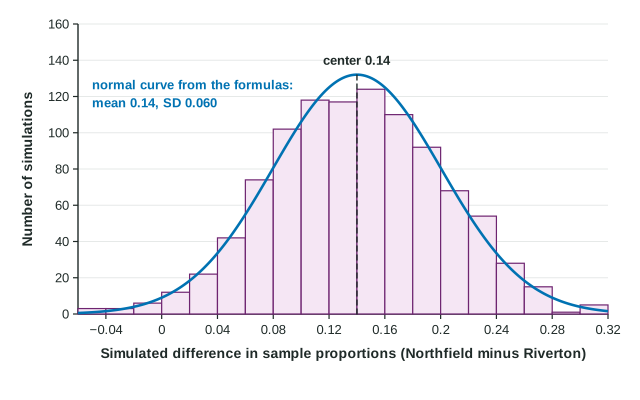
Histogram of 1,000 simulated differences in sample proportions, Northfield minus Riverton, centered at 0.14 and running from about 0 to 0.30, with a normal curve of mean 0.14 and standard deviation 0.060 drawn over the bars. — **Figure 1.** 1,000 simulated differences $\hat{p}_A - \hat{p}_B$ for samples of 150 and 120, with the normal curve from the formulas. LevlPrep original diagram.

In Northfield, 62% of households compost; in Riverton, 48% do. The figure shows 1,000 simulated values of $\hat{p}_A - \hat{p}_B$ for random samples of 150 Northfield and 120 Riverton households. The bars pile up around 0.14, the true difference, and the normal curve from the formulas fits them well. Most differences land between about 0.02 and 0.26, roughly two standard deviations either side of the center.

Worked example. For the compost samples, find the probability that the sample difference $\hat{p}_A - \hat{p}_B$ is 0 or less, so that the sample makes Riverton look at least as good as Northfield.

Center: $\mu = 0.62 - 0.48 = 0.14$ .

Spread: $\sigma$ $= \sqrt{\frac{0.62(0.38)}{150} + \frac{0.48(0.52)}{120}}$ $= \sqrt{0.00157 + 0.00208}$ $= \sqrt{0.00365}$ $= 0.060$ .

Shape: $150(0.62) = 93$ , $150(0.38) = 57$ , $120(0.48) = 57.6$ and $120(0.52) = 62.4$ are each at least 10, so the distribution is approximately normal. The samples are independent and random, and each is far less than 10% of the households in its town.

Probability: $z$ $= \frac{0 - 0.14}{0.060}$ $= -2.32$ , and the area to the left under the standard normal curve is about $0.010$ .

In context: only about 1% of pairs of samples like these would show Riverton composting at least as much as Northfield. A sample like that would be surprising if the true rates really are 62% and 48%.

Why this matters next

In the next topics you will not know $p_1$ and $p_2$ ; you will estimate their difference with an interval and test whether it is 0. Both tools stand on this sampling distribution: its center tells you the difference is unbiased, and its standard deviation tells you how far a sample difference typically lands from the truth.