Two-Proportion Sampling Distribution

Part 1 · Hook

Why this matters

A district says 70% of its high schoolers ride the bus but only 55% of its middle schoolers do. A reporter checks with two random samples and gets a gap of 0.02 instead of 0.15. Is the district wrong, or is that just what samples do? To answer, you need to know how a difference of two sample proportions behaves from sample to sample.

Part 2 · Before you start

What this builds on

Part 3 · Prerequisite check

Quick check before you start

1. A population has $p = 0.4$ . What is the standard deviation of $\hat{p}$ for random samples of 100?

$0.049$
$0.0024$
$0.24$
$0.4$

Show the answer

$\sqrt{\frac{0.4(0.6)}{100}}$ $= \sqrt{0.0024}$ $= 0.049$ .

Correct: $0.049$ :
$0.0024$ :
$0.24$ :
$0.4$ :

2. For $n = 50$ and $p = 0.1$ , is the large counts condition met?

No: $50(0.1) = 5$ is less than 10
Yes: $n = 50$ is at least 30
Yes: $50(0.9) = 45$ is at least 10
No: $p$ is less than 0.5

Show the answer

Both $np$ and $n(1 - p)$ must be at least 10; $np = 5$ fails.

Correct: No: $50(0.1) = 5$ is less than 10:
Yes: $n = 50$ is at least 30:
Yes: $50(0.9) = 45$ is at least 10:
No: $p$ is less than 0.5:

3. A normal distribution has mean 0.15 and standard deviation 0.05. What is the z-score of 0.05?

$-2$
$2$
$-0.1$
$-1$

Show the answer

$z$ $= \frac{0.05 - 0.15}{0.05}$ $= -2$ .

Correct: $-2$ :
$2$ :
$-0.1$ :
$-1$ :

Part 4 · See it

See it first

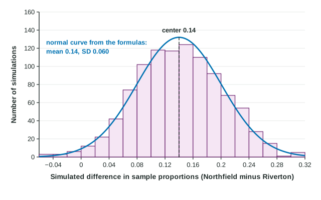
Histogram of 1,000 simulated differences in sample proportions, Northfield minus Riverton, centered at 0.14 and running from about 0 to 0.30, with a normal curve of mean 0.14 and standard deviation 0.060 drawn over the bars. — 1,000 simulated values of $\hat{p}_A - \hat{p}_B$ with the normal curve the formulas predict: mean 0.14, standard deviation 0.060. LevlPrep original diagram.

Part 5 · Step by step

How it works, step by step

Take a random sample from each of two populations, independentlyeach sample proportion has its own chance error, and so does their difference $\hat{p}_1 - \hat{p}_2$
Each sample proportion is centered at its true proportionthe difference is centered at $p_1 - p_2$ , so it is an unbiased estimator of the true difference
The two chance errors come from separate samples and do not cancelthe variances add: $\sigma^2$ $= \frac{p_1(1-p_1)}{n_1}$ $+ \frac{p_2(1-p_2)}{n_2}$ , and the standard deviation is its square root
Both samples have at least 10 expected successes and 10 expected failuresthe sampling distribution is approximately normal, so z-scores and normal areas give probabilities

Part 6 · Key ideas

Key ideas

Mean: $\mu_{\hat{p}_1 - \hat{p}_2}$ $= p_1 - p_2$ .
Standard deviation: $\sigma_{\hat{p}_1 - \hat{p}_2}$ $= \sqrt{\frac{p_1(1-p_1)}{n_1} + \frac{p_2(1-p_2)}{n_2}}$ . Add variances, never standard deviations.
Shape: approximately normal when $n_1 p_1$ , $n_1(1-p_1)$ , $n_2 p_2$ and $n_2(1-p_2)$ are each at least 10.
Conditions: two independent random samples (or two randomly assigned groups), and each sample less than 10% of its population when sampling without replacement.

Part 7 · Misconception

A common mistake

The wrong idea: Subtracting the sample proportions means you subtract their standard deviations too, so the difference varies less than either one.

What actually happens: Each sample brings its own chance error, and the errors add up rather than cancel. The variances add, so a difference varies more than either sample proportion alone.

Part 8 · Check yourself

Check yourself

Exam-style questions. Anything you miss goes into your review queue.

Table

Bus riders in two school levels

A school district knows from its bus card records that 70% of its high school students and 55% of its middle school students ride a district bus at least once a week. A reporter takes independent random samples of 100 high school students and 80 middle school students and finds the sample proportion of bus riders in each,

\hat{p}_H

and

\hat{p}_M

. (Invented data.)

Population proportions and sample sizes
Group	Proportion who ride	Sample size
High school	0.70	100
Middle school	0.55	80

1. What is the mean of the sampling distribution of $\hat{p}_H - \hat{p}_M$ ?

$0.625$
$1.27$
$0$
$0.15$

Show the answer

The difference $\hat{p}_H - \hat{p}_M$ is an unbiased estimator of $p_H - p_M = 0.15$ .

$0.625$ : That averages the two proportions. The distribution of a difference is centered at the difference, $0.70 - 0.55$ .
$1.27$ : That divides 0.70 by 0.55. A difference is centered at $p_H - p_M$ , a subtraction, not a ratio.
$0$ : Zero would be the mean only if the two population proportions were equal. Here they differ by 0.15.
Correct: $0.15$ : Right: the mean of a difference in sample proportions is the difference in the population proportions, $0.70 - 0.55 = 0.15$ .

2. What is the standard deviation of the sampling distribution of $\hat{p}_H - \hat{p}_M$ ? Give three decimal places.

Type a number. A table answer and a calculator answer are both accepted.

Show the answer

$\sigma$ $= \sqrt{\frac{0.70(0.30)}{100} + \frac{0.55(0.45)}{80}}$ $= \sqrt{0.0021 + 0.00309}$ $= 0.072$ .

Answer: 0.072

3. Which check shows that the sampling distribution of $\hat{p}_H - \hat{p}_M$ is approximately normal?

Both population proportions, 0.70 and 0.55, are above 0.5
Both samples were selected at random from the district
$100(0.70) = 70$ , $100(0.30) = 30$ , $80(0.55) = 44$ and $80(0.45) = 36$ are each at least 10
The combined sample size, $100 + 80 = 180$ , is at least 30

Show the answer

Approximate normality needs at least 10 expected successes and 10 expected failures in each sample.

Both population proportions, 0.70 and 0.55, are above 0.5: Proportions above 0.5 do not make a shape normal. The counts $n p$ and $n(1 - p)$ in each sample must reach 10.
Both samples were selected at random from the district: Random selection lets you generalize, but it says nothing about the shape. The shape comes from the large counts condition.
Correct: $100(0.70) = 70$ , $100(0.30) = 30$ , $80(0.55) = 44$ and $80(0.45) = 36$ are each at least 10: Right: the large counts condition is checked for both samples, successes and failures, four counts in all.
The combined sample size, $100 + 80 = 180$ , is at least 30: Comparing $n$ with 30 is a rule for sample means. For proportions, check the four counts $n_1 p_1$ , $n_1(1 - p_1)$ , $n_2 p_2$ , $n_2(1 - p_2)$ against 10.

4. What is the probability that $\hat{p}_H - \hat{p}_M$ is 0.05 or less? Give four decimal places.

Type a number. A table answer and a calculator answer are both accepted.

Show the answer

$z$ $= \frac{0.05 - 0.15}{0.072}$ $= -1.39$ , so $P(\hat{p}_H - \hat{p}_M \le 0.05)$ $= 0.0826$ (the area to the left of $z$ under the standard normal curve).

Answer: 0.0826

5. In a large city, 35% of adults under 30 and 25% of adults 30 or older use a bike share at least once a month. Independent random samples of 250 younger adults and 200 older adults are taken. Write the expression for the standard deviation of $\hat{p}_{\text{young}} - \hat{p}_{\text{old}}$ , then give its value to three decimal places.

Type the expression as on the exam, with the values substituted.

Show the answer

$\sigma$ $= \sqrt{\frac{0.35(0.65)}{250} + \frac{0.25(0.75)}{200}}$ $= \sqrt{0.00091 + 0.00094}$ $= 0.043$ .

Answer: $\sqrt{\frac{0.35 \cdot 0.65}{250} + \frac{0.25 \cdot 0.75}{200}}$

6. Which change makes the standard deviation of $\hat{p}_1 - \hat{p}_2$ smaller, with the population proportions kept the same?

Using a larger difference between the populations
Combining the two samples into one
Subtracting in the other order, $\hat{p}_2 - \hat{p}_1$
Taking larger samples from both populations

Show the answer

Both terms $\frac{p(1-p)}{n}$ shrink as their $n$ grows.

Using a larger difference between the populations: The question keeps the proportions fixed. The spread is lowered by larger samples.
Combining the two samples into one: One combined sample gives one proportion. It no longer measures a difference between two groups.
Subtracting in the other order, $\hat{p}_2 - \hat{p}_1$ : Switching the order changes the sign of the mean, not the spread. The variances add either way.
Correct: Taking larger samples from both populations: Right: each variance term has its sample size in the denominator, so larger samples shrink both terms.

Part 9 · Summary

Summary

For two independent random samples,

\hat{p}_1 - \hat{p}_2

is centered at

p_1 - p_2

and has standard deviation

\sqrt{\frac{p_1(1-p_1)}{n_1} + \frac{p_2(1-p_2)}{n_2}}

: the variances add. When all four large counts are at least 10, its distribution is approximately normal, so you can find probabilities with z-scores.

Part 10 · Up next

What comes next

Part 11 · Connections