Sampling Distributions and the Central Limit Theorem

Take a random sample, compute a statistic, and you get one number. Take another random sample from the same population and you will get a slightly different number. This topic is about that variation: how much a statistic changes from sample to sample, and what pattern the changes follow. It is the idea that makes inference in Units 3 and 4 possible.

Statistics vary: sampling variability

In a large city, 40% of voters support a park tax. That 0.40 is a parameter: one fixed number describing every voter. Poll a random sample of 100 voters and the sample proportion $\hat{p}$ might be 0.37. Another sample might give 0.44. A statistic varies from sample to sample because each sample holds different individuals. This is sampling variability, and it is not a mistake: it happens even with perfect random sampling.

The sampling distribution of a statistic is the distribution of its values in all possible random samples of the same size from the same population. We rarely see it directly, but a simulation can approximate it: a computer took 500 random samples of 100 voters and the 500 values of $\hat{p}$ pile up around 0.40, mostly between about 0.30 and 0.50, in a roughly symmetric mound.

Three distributions, kept apart

Most confusion in this topic comes from mixing these up. The sample looks like the population (skewed if the population is skewed). The sampling distribution is a different object: a distribution of means or proportions.

Center and spread of the sampling distribution of $\bar{x}$

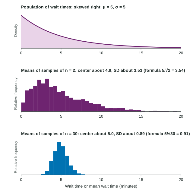
Pharmacy wait times are strongly skewed right with mean $\mu = 5$ minutes and standard deviation $\sigma = 5$ minutes. The figure shows simulated sample means for two sample sizes. Two patterns hold for any sample size n:

• Center: $\mu_{\bar{x}} = \mu$. Sample means are centered at the population mean; they do not systematically run high or low.
• Spread: $\sigma_{\bar{x}} = \frac{\sigma}{\sqrt{n}}$. Averaging more individuals cancels out more of the extreme values, so the means vary less.

For samples of 40 waits, $\sigma_{\bar{x}}$$= \frac{5}{\sqrt{40}}$$\approx 0.79$ minutes, much less than the 5-minute spread of single waits. Because of the square root, quadrupling the sample size halves the spread. The same ideas hold for $\hat{p}$: its sampling distribution is centered at p, and larger samples make it less variable. Unit 3 gives the formula for its spread.

Shape: the Central Limit Theorem

If the population is normal, the sampling distribution of $\bar{x}$ is normal for any sample size. If the population is not normal, something remarkable happens anyway. The Central Limit Theorem says that when n is large, the sampling distribution of $\bar{x}$ is approximately normal, whatever the shape of the population. In the figure, means of 2 waits are still skewed right, but means of 30 waits form a near bell shape. A common guide is that n of 30 or more is large enough; strongly skewed populations need larger samples than mildly skewed ones.

The theorem is about the sample mean, not the data. A sample of 1,000 waits is still skewed right. It is the means of many samples that pile up in a normal shape.

Using the sampling distribution

The same calculation can test a claim. If a random sample of 40 had a mean wait of 7.5 minutes, then $z$$= \frac{7.5 - 5}{0.791}$$\approx 3.16$ and $P(\bar{x} \ge 7.5) \approx 0.0008$. If the pharmacy's numbers were right, a sample mean that high would almost never happen, so the sample gives strong reason to doubt them. That reasoning, "how surprising is this statistic if the claim is true?", is the core of the inference methods in Units 3 and 4.

The common slip is using $\sigma$ in place of $\sigma_{\bar{x}}$. Single waits of 6 minutes or more are common; sample means of 40 waits that high are not, because means vary much less than individuals.