Unit 2 · Topic 2.12 Beta

Sampling Distributions and the Central Limit Theorem

A statistic varies from sample to sample, and its sampling distribution describes how.

Practice 4: Interpret Results

Part 1 · Hook

Why this matters

A pharmacy says customers wait 5 minutes on average. You time 40 customers and get an average of 7.5 minutes. Bad luck, or a false claim? Every sample gives a slightly different average, so the question is how much averages bounce around. The answer, the sampling distribution, is the bridge to everything in Units 3 and 4.

Part 2 · Before you start

What this builds on

Part 3 · Prerequisite check

Quick check before you start

1. Which is a statistic?

The mean height of 50 sunflowers in a sample
The mean height of all sunflowers in the field
The number of sunflowers in the field
The true proportion of tall sunflowers

Show the answer

A statistic describes a sample.

Correct: The mean height of 50 sunflowers in a sample:
The mean height of all sunflowers in the field:
The number of sunflowers in the field:
The true proportion of tall sunflowers:

2. For $N(5, 0.8)$ , what is the z-score of 7.4?

3
2.4
0.33
9.25

Show the answer

$\frac{7.4 - 5}{0.8} = 3$ .

Correct: 3:
2.4:
0.33:
9.25:

Part 4 · See it

See it first

A skewed population of wait times, then 2000 sample means for n = 2 and for n = 30. The means center at 5, spread less as n grows, and become bell-shaped. LevlPrep original diagram.

Part 5 · Step by step

How it works, step by step

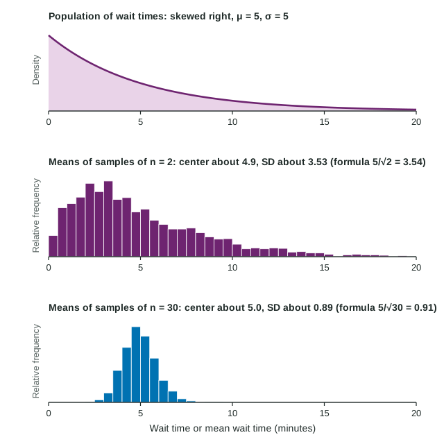
Different random samples contain different individualsa statistic such as $\bar{x}$ or $\hat{p}$ varies from sample to sample (sampling variability)
Collect the statistic from every possible sample of size nits sampling distribution, with a center, a spread and a shape
Average more individuals in each samplethe center stays at the parameter, $\mu_{\bar{x}} = \mu$ , and the spread shrinks, $\sigma_{\bar{x}} = \frac{\sigma}{\sqrt{n}}$
Make n large, even from a skewed populationthe Central Limit Theorem makes the sampling distribution of $\bar{x}$ approximately normal

Part 6 · Key ideas

Key ideas

A statistic varies from sample to sample. Its sampling distribution is the distribution of its values over all possible random samples of the same size.
Keep three distributions apart: the population, one sample's data, and the sampling distribution of a statistic.
For $\bar{x}$ : center $\mu_{\bar{x}} = \mu$ and spread $\sigma_{\bar{x}} = \frac{\sigma}{\sqrt{n}}$ . Four times the sample size halves the spread. For $\hat{p}$ , the center is p.
The Central Limit Theorem: for large n (a common guide is 30 or more), the sampling distribution of $\bar{x}$ is approximately normal whatever the population's shape. A normal population gives normal $\bar{x}$ at any n.

Part 7 · Misconception

A common mistake

The wrong idea: The Central Limit Theorem says a large sample of data looks normal.

What actually happens: A large sample from a skewed population is still skewed. The CLT is about the sample mean: across many samples, the values of $\bar{x}$ pile up in a roughly normal shape.

Part 8 · Check yourself

Check yourself

Exam-style questions. Anything you miss goes into your review queue.

Graph

Simulated sample means of wait times

Wait times at a pharmacy counter are strongly skewed right, with mean 5 minutes and standard deviation 5 minutes. A computer took 200 random samples of 5 customers and 200 random samples of 40 customers and found the mean wait time of each sample. The boxplots show the 200 sample means for each sample size (simulated data).

1. How do the centers of the two distributions of sample means compare?

The n = 40 means are centered much higher, because larger samples catch more long waits
The n = 5 means are centered near 1 minute, the most common single wait
Both are centered near 5 minutes, the population mean
The n = 40 means are centered near 40 minutes, the sample size

Show the answer

Both are centered near 5 minutes (medians 4.32 and 4.84; means 4.91 and 5.01), the population mean: the mean of the sampling distribution of $\bar{x}$ is $\mu$ , whatever the sample size.

The n = 40 means are centered much higher, because larger samples catch more long waits: A larger sample does not move the center; it shrinks the spread.
The n = 5 means are centered near 1 minute, the most common single wait: Sample means are centered at the population mean, 5 minutes.
Correct: Both are centered near 5 minutes, the population mean: Right: $\mu_{\bar{x}} = \mu$ for any sample size.
The n = 40 means are centered near 40 minutes, the sample size: The sample size sets the spread, not the center.

2. How do the spreads compare?

The n = 40 means are more spread out, because there are more customers in each sample
The spreads are about the same, because both used 200 samples
The n = 5 means have no spread, because each is an average
The n = 40 means are much less spread out than the n = 5 means

Show the answer

The means of samples of 40 vary much less (SD about 0.84 minutes) than the means of samples of 5 (about 2.4). The formula $\sigma_{\bar{x}} = \frac{\sigma}{\sqrt{n}}$ gives $\frac{5}{\sqrt{5}} \approx 2.24$ and $\frac{5}{\sqrt{40}} \approx 0.79$ .

The n = 40 means are more spread out, because there are more customers in each sample: More customers per sample average out more, so the means vary less.
The spreads are about the same, because both used 200 samples: The number of samples does not set the spread; the sample size does.
The n = 5 means have no spread, because each is an average: Averages of 5 values still vary from sample to sample.
Correct: The n = 40 means are much less spread out than the n = 5 means: Right: larger samples give less variable sample means.

3. What is the standard deviation of the sampling distribution of $\bar{x}$ for samples of 40 customers, in minutes?

Type a number. A table answer and a calculator answer are both accepted.

Show the answer

$\sigma_{\bar{x}}$ $= \frac{\sigma}{\sqrt{n}}$ $= \frac{5}{\sqrt{40}}$ $\approx 0.79$ minutes.

Answer: 0.79

4. The population of wait times is strongly skewed right. What about the shapes of the two distributions of sample means?

Both are skewed right, since the population is skewed right
n = 5: still skewed right; n = 40: close to symmetric
Both are exactly normal, since they are made of means
The n = 5 means are symmetric and the n = 40 means are skewed

Show the answer

With n = 5 the sample means are still skewed right, with high outliers. With n = 40 they are close to symmetric: by the Central Limit Theorem, the sampling distribution of $\bar{x}$ is approximately normal when n is large.

Both are skewed right, since the population is skewed right: The skew fades as n grows; with n = 40 the means are close to symmetric.
Correct: n = 5: still skewed right; n = 40: close to symmetric: Right: the Central Limit Theorem at work as n grows.
Both are exactly normal, since they are made of means: Means of small samples from a skewed population keep some skew.
The n = 5 means are symmetric and the n = 40 means are skewed: It is the other way around: more averaging means less skew.

5. What is the sampling distribution of a statistic?

The distribution of the data values in one random sample
The distribution of the values in the whole population
The list of sampling methods, such as stratified or cluster, a study could use
The distribution of its values in all possible random samples of the same size

Show the answer

The sampling distribution is the distribution of the values a statistic takes in all possible random samples of the same size from the same population.

The distribution of the data values in one random sample: That is the distribution of a sample, not of a statistic.
The distribution of the values in the whole population: That is the population distribution.
The list of sampling methods, such as stratified or cluster, a study could use: Sampling methods are a design choice, not a distribution.
Correct: The distribution of its values in all possible random samples of the same size: Right: it shows how the statistic varies from sample to sample.

6. Which statement is the Central Limit Theorem?

For large n, $\bar{x}$ has an approximately normal sampling distribution
When n is large, the data values in one sample are approximately normal in shape
When n is large, the population becomes approximately normal
When n is large, the sample mean equals the population mean

Show the answer

The CLT is about sample means: when n is large, the sampling distribution of $\bar{x}$ is approximately normal, whatever the shape of the population. A common guide is n of 30 or more.

Correct: For large n, $\bar{x}$ has an approximately normal sampling distribution: Right: the shape of $\bar{x}$ , not of the data.
When n is large, the data values in one sample are approximately normal in shape: A sample from a skewed population stays skewed, however large.
When n is large, the population becomes approximately normal: Sampling does not change the population.
When n is large, the sample mean equals the population mean: The sample mean still varies; it just varies less.

Part 9 · Summary

Summary

A statistic varies from sample to sample, and its sampling distribution describes how. For the sample mean, the center is

\mu

and the spread is

\frac{\sigma}{\sqrt{n}}

, so larger samples give less variable means. By the Central Limit Theorem, for large n the sampling distribution of

\bar{x}

is approximately normal even from a skewed population, which lets you judge whether a sample mean is surprising.

Part 10 · Up next

What comes next

Part 11 · Connections

Connections

Question set for this topic