Topic 1.6 described center and spread by eye. This topic gives them numbers: the mean and median for center; the range, IQR and standard deviation for spread; quartiles and percentiles for position; and two rules for deciding what counts as an outlier. The key idea running through all of them is which summaries an extreme value can push around.
Measures of center: mean and median
The mean is the sum of the values divided by how many there are. For a sample it is written ("x-bar"):
The median is the middle of the ordered values. With an odd number of values it is the middle one; with an even number it is the average of the two middle ones. Half the data are at or below the median.
Mean and median. The battery lives, in hours, of 12 phones in order: 7.2, 8.1, 8.4, 8.9, 9.0, 9.3, 9.5, 9.8, 10.1, 10.4, 10.6, 14.9.
Mean:
Median: is even, so average the 6th and 7th values: hours.
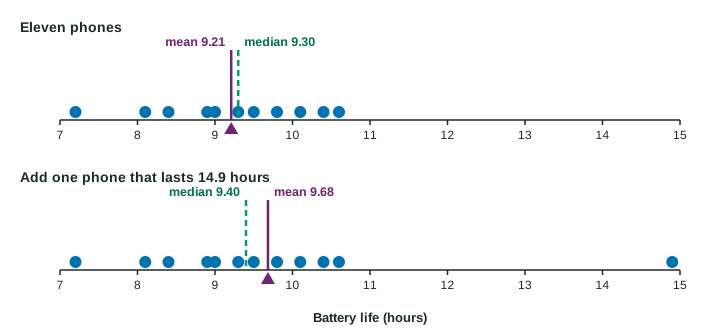
Why are they different? The mean uses every value, so the one phone at 14.9 hours drags it up. The median only cares about order: make that phone last 30 hours and the median stays at 9.4. A summary that extreme values barely change is called resistant. The median is resistant; the mean is not. So the mean is pulled toward a long tail: in a right-skewed distribution the mean is usually larger than the median, and in a left-skewed one it is usually smaller.
Quartiles, percentiles and the IQR
The quartiles split the ordered data into quarters. is the median of the lower half and is the median of the upper half. When n is odd, leave the median itself out of both halves (this is the method the exam uses, and the one technology here uses).
The interquartile range, , is the spread of the middle half of the data. The range is maximum minus minimum. Both are single numbers: write "the range is 7.7 hours", not "the range is 7.2 to 14.9".
A percentile gives position: the pth percentile is the value with p% of the data at or below it. is about the 25th percentile, the median the 50th, the 75th. A score at the 80th percentile is not 80% correct; it is a score that 80% of the scores are at or below.
Standard deviation
The standard deviation measures the typical distance of the values from the mean. Its recipe: find each distance from the mean, square it, add the squares, divide by , and take the square root.
Why square? The distances above and below the mean always add to 0, so they would cancel. Squaring makes each one count. Why divide by and not ? A sample’s values sit a little closer to their own mean than to the population mean, so the squared distances run a little small; dividing by makes up for that. The square of the standard deviation, , is the variance.
A standard deviation by hand. The values 4, 6, 11 have mean .
Distances: , , . Squares: 9, 1, 16, which add to 26.
For the 12 phones, technology gives hours: battery lives typically differ from the mean of 9.68 hours by about 1.9 hours.
The standard deviation is 0 only when every value is the same, and it is not resistant: one far-out value adds a huge squared distance. For a whole population the mean and standard deviation are written and ; for a sample, and .
Two rules for outliers
- The rule. A value is an outlier if it is below or above . These two cutoffs are the fences.
- The 2 standard deviation rule. A value more than 2 standard deviations from the mean is flagged as unusual.
Use the fences. For the 12 phones: lower half 7.2 to 9.3, so
Lower fence: . Upper fence: .
Only 14.9 hours is beyond a fence, so it is the one outlier. In context: "The phone that lasted 14.9 hours is an outlier, since it is above the upper fence of 12.65 hours."
Which summaries to report
| Resistant | Not resistant | |
|---|---|---|
| Center | median | mean |
| Spread | IQR | standard deviation, range |
| Report when | the distribution is skewed or has outliers | the distribution is roughly symmetric with no outliers |
Changing units
If you add the same constant to every value, every measure of center and position (mean, median, quartiles) shifts by that constant, and every measure of spread (range, IQR, standard deviation) stays the same: the values all move together. If you multiply every value by a constant, center, position and spread are all multiplied by it. Five plants grew 4, 5, 6, 8 and 12 inches, with mean 7 and standard deviation 3.16 inches. In centimeters () the mean is cm and the standard deviation is cm.