Some random variables are measurements rather than counts: an egg's weight, a battery's life, a person's height. They can take any value in a range, so there is no list of values to put in a table. Instead, a smooth curve describes the distribution, and probabilities are areas under it. The most important such curve is the normal curve.
Density curves
A density curve is a smooth curve that lies on or above the horizontal axis and has an area of exactly 1 under it. The area over any interval is the proportion of values in that interval, which is also the probability that a randomly chosen value lands there. It is like a histogram with very narrow bars, rescaled so the total area is 1.
One consequence surprises people: the probability of any single exact value is 0, because a single point has no width and so no area. is 0; is not. For the same reason, and are equal for a continuous random variable.
Normal distributions
A normal distribution has a symmetric, single-peaked, bell-shaped density curve. Two parameters fix it: the mean , at the center, and the standard deviation , which sets the spread. Write it . Egg weights at a farm might be grams. The curve changes from bending down to bending up one standard deviation from the mean on each side, at 54 and 62 grams.
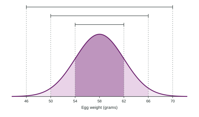
Every normal curve has the same shape when measured in standard deviations, which gives the empirical rule, shown in the figure:
- about 68% of values lie within 1 standard deviation of the mean (54 to 62 grams);
- about 95% lie within 2 standard deviations (50 to 66 grams);
- about 99.7% lie within 3 standard deviations (46 to 70 grams).
Because the curve is symmetric, the leftover 5% outside 2 standard deviations splits evenly: about 2.5% of eggs weigh more than 66 grams.
A normal model is a model, not a law. It fits many roughly symmetric, mound-shaped distributions. It does not fit strongly skewed data, like bank waiting times, whatever their mean and standard deviation.
Standardizing: the standard normal
For values that are not a whole number of standard deviations away, standardize. The z-score from Unit 1, , says how many standard deviations a value is from the mean. Standardizing a normal random variable gives the standard normal distribution, . Table A on the reference sheet lists the area to the left of each z from about −3.4 to 3.4; a calculator's normal area command gives the same areas directly.
Worked example 1. Battery life B is hours. Find the probability that a battery lasts less than 16 hours.
Name the distribution, boundary and direction: B is ; we want , the area to the left of 16. A sketch shades the left tail.
Standardize:
Find the area: from Table A (technology, without rounding z: 0.0912). About 9% of batteries last less than 16 hours.
For an area to the right, subtract from 1:
Working backward: from an area to a value
Sometimes the area is given and the boundary is wanted, such as a percentile or a cutoff. Reverse the steps: find the z with the right area to its left (Table A read from the inside out, or an inverse normal command), then turn it back into the original units with .
Worked example 2. The heaviest 5% of eggs are sold as jumbo. Find the minimum jumbo weight.
The boundary has 95% of the area below it, so .
Unstandardize: grams. Eggs of about 64.6 grams or more are jumbo.
Show the work the exam asks for
A calculator command on its own ("normalcdf") does not earn credit. Write the distribution and its parameters, the boundary, and the direction, with a labeled sketch or in symbols: "W is ;
| Question | Steps |
|---|---|
| Area from a value | name , sketch, , area to the left (subtract from 1 for the right) |
| Area between two values | two z-scores, subtract the two left areas |
| Value from an area | area to the left, inverse normal z, |
| Comparing two values on different scales | compare z-scores, not raw values |