Parameters of Random Variables — AP® Statistics Notes

In Unit 1 you summarized a data set with its mean and standard deviation. A probability distribution can be summarized the same way. The only change is that values are weighted by their probabilities instead of counted equally. These two numbers, the mean and standard deviation of a random variable, describe what happens in the long run.

The mean, or expected value

Let X = the number of tacos in a randomly chosen order at a food truck.

$x$	1	2	3	4	5
$P(X = x)$	0.20	0.35	0.25	0.15	0.05

Imagine 100 typical orders: about 20 have 1 taco, 35 have 2, 25 have 3, 15 have 4 and 5 have 5. The total is $20 + 70 + 75 + 60 + 25$ $= 250$ tacos, or 2.5 tacos per order. Dividing by 100 at the end is the same as multiplying each value by its probability. That gives the formula for the mean or expected value of a discrete random variable, which is on the reference sheet:

$\mu_X = E(X) = \sum x_i p_i.$

Worked example 1. Find the mean of X.

Structure: $\mu_X = \sum x_i p_i$ .

Substitute: $1(0.20)$ $+ 2(0.35)$ $+ 3(0.25)$ $+ 4(0.15)$ $+ 5(0.05)$ $= 0.20$ $+ 0.70$ $+ 0.75$ $+ 0.60$ $+ 0.25$ .

Answer: $\mu_X = 2.5$ tacos. Interpretation: over many orders, the average number of tacos per order is about 2.5.

Three things to notice. The mean is not the plain average of 1 to 5 (that would be 3): small orders are more likely, so they pull the mean down. The mean need not be a possible value: no order contains 2.5 tacos. And it is a long-run statement: it does not predict the next order.

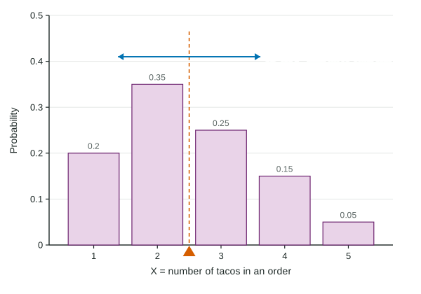
Probability histogram of X, the number of tacos in an order: 0.20, 0.35, 0.25, 0.15 and 0.05 for 1 to 5 tacos. A triangle under the axis marks the mean, 2.5 tacos, where the histogram would balance; arrows show one standard deviation, about 1.12 tacos, on each side. — **Figure 1.** The mean is the balance point of the probability histogram. LevlPrep original diagram.

Picture the probability histogram as a seesaw with weights on it. The mean is where it balances, as in the figure.

The standard deviation

The standard deviation of X measures how far its values typically fall from the mean. Weight each squared distance from the mean by its probability, add, and take the square root:

$\sigma_X = \sqrt{\sum (x_i - \mu_X)^2 p_i}.$

Worked example 2. Find the standard deviation of X.

Structure: $\sigma_X$ $= \sqrt{\sum (x_i - \mu_X)^2 p_i}$ with $\mu_X = 2.5$ .

Substitute: $(1 - 2.5)^2(0.20)$ $+ (2 - 2.5)^2(0.35)$ $+ (3 - 2.5)^2(0.25)$ $+ (4 - 2.5)^2(0.15)$ $+ (5 - 2.5)^2(0.05)$ $= 0.45$ $+ 0.0875$ $+ 0.0625$ $+ 0.3375$ $+ 0.3125$ $= 1.25$ .

Answer: $\sigma_X = \sqrt{1.25} \approx 1.12$ tacos. Interpretation: the number of tacos in an order typically differs from the mean of 2.5 by about 1.12 tacos.

The number inside the square root, 1.25, is the variance. Forgetting the square root is a common slip; the standard deviation is in tacos, the same units as X. Unlike a sample's standard deviation, there is no $n - 1$ here: the probabilities already are the weights.

Expected gain in games and insurance

Expected value is how fundraisers, casinos and insurers plan. A school game costs $2. It pays $10 with probability 0.10 and $5 with probability 0.15. Let W = a player's net gain: $8, $3 or −$2.

$\mu_W = 8(0.10) + 3(0.15) + (-2)(0.75) = 0.80 + 0.45 - 1.50 = -0.25.$

Interpretation: if many people play, players lose an average of about 25 cents per play, so the school raises about $0.25 per play in the long run, roughly $100 over 400 plays. A game is fair when the expected net gain is 0.

Common slips

Slip	Fix
Averaging the values, $\frac{1 + 2 + 3 + 4 + 5}{5}$	weight each value by its probability
Averaging the probabilities	the probabilities alone always add to 1; multiply by the values
Reporting the variance as the SD	take the square root
Prizes instead of net gains	subtract the cost from every prize, including the $0 prize
Only the answer, no expression	write $\sum x_i p_i$ with every number substituted

Comparing spreads works as with data: two random variables with the same mean can have very different standard deviations. Values farther from the mean, with the same probabilities, mean a larger $\sigma$ .