Potential Errors When Performing… — AP® Statistics Notes

A significance test makes a decision from a sample, and samples vary. So even a test done perfectly can reach the wrong decision. This topic names the two ways a test can be wrong, says how likely each one is, and shows what you can do about them. The exam asks you to describe each error in context and to explain its consequence.

Two ways to be wrong

The truth is either $H_0$ or $H_a$ , and the decision is either reject $H_0$ or fail to reject it. That gives four outcomes, two of them mistakes.

	$H_0$ is true	$H_a$ is true
Reject $H_0$	Type I error (probability $\alpha$ )	Correct (probability = power)
Fail to reject $H_0$	Correct	Type II error (probability $\beta$ )

A Type I error is rejecting $H_0$ when $H_0$ is true: finding convincing evidence for an effect that is not there.
A Type II error is failing to reject $H_0$ when $H_a$ is true: missing an effect that is there.

Only one error is possible after a decision. If you rejected $H_0$ , the only possible mistake is Type I. If you failed to reject, the only possible mistake is Type II.

Describing an error in context

Readers want the condition first: what is actually true, then the wrong decision, then what happens because of it.

Worked example. A city must replace its water pipes if more than 10% of its homes have lead above a safety limit. It tests $H_0: p = 0.10$ against $H_a: p > 0.10$ , where $p$ is the true proportion of all the city's homes with lead above the limit, and replaces the pipes if there is convincing evidence for $H_a$ . Describe each error and its consequence.

Type I error. The true proportion of all the city's homes with lead above the limit is 0.10, but the test finds convincing evidence that it is greater than 0.10. Consequence: the city spends money replacing pipes that did not need replacing.

Type II error. The true proportion of all the city's homes with lead above the limit is greater than 0.10, but the test does not find convincing evidence that it is greater than 0.10. Consequence: the pipes are not replaced, and residents keep drinking water with too much lead.

Which is worse? Here the Type II error is a health risk, so the city should make it less likely, for example by using $\alpha = 0.10$ instead of 0.01 or by testing more homes.

How likely is each error?

Type I. If $H_0$ is true, the test rejects whenever the p-value falls below $\alpha$ , and that happens with probability $\alpha$ . So $P(\text{Type I error}) = \alpha$ . Choosing $\alpha$ is choosing how often you are willing to raise a false alarm.

Type II. Its probability, $\beta$ , depends on what the true value of $p$ actually is. A true proportion of 0.11 is hard to tell apart from 0.10; a true proportion of 0.20 is easy. So $\beta$ is always "against" a specific alternative value.

The power of a test against a specific alternative is the probability that it rejects $H_0$ when that alternative is true: the chance it detects a real effect. $\text{power} = 1 - \beta$ .

Seeing α, β and power

Two normal curves for the sample proportion from samples of 200. The left curve, centered at the null value 0.50, is the distribution if the null is true; the right curve, centered at 0.60, is the distribution if the true proportion is 0.60. A vertical line at the cutoff 0.558 marks where the test rejects H0 at alpha = 0.05 (sample proportions above it). Under the null curve, the small area beyond the cutoff is alpha, the probability of a Type I error. Under the alternative curve, the area to the left of the cutoff is beta, the probability of a Type II error, about 0.11; the area to the right is the power, about 0.89. — **Figure 1.** A one-sided test of H0: p = 0.5 with 200 customers at α = 0.05 rejects when the sample proportion is 0.558 or more. If p is really 0.60, the area beyond the cutoff under the right curve is the power, about 0.89; the area before it is β, about 0.11. LevlPrep original diagram.

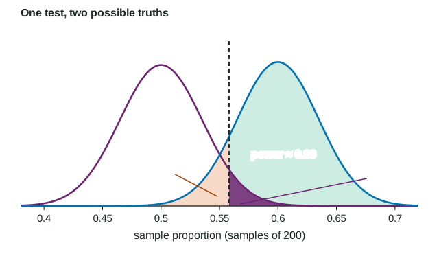
A snack company will switch recipes only if there is convincing evidence that more than half of its customers prefer the new one. With 200 customers and $\alpha = 0.05$ , the test rejects $H_0: p = 0.5$ when $\hat{p} \ge 0.5$ $+ 1.645\sqrt{\frac{0.5(0.5)}{200}}$ $= 0.558$ . If in fact $p = 0.60$ , then $\hat{p}$ is approximately normal with mean 0.60 and standard deviation $\sqrt{\frac{0.60(0.40)}{200}}$ $= 0.0346$ , and

$\text{power} = P(\hat{p} \ge 0.558) = P\left(Z \ge \frac{0.558 - 0.60}{0.0346}\right) = P(Z \ge -1.21) = 0.887.$

So $\beta = 1 - 0.887 = 0.113$ : about an 11% chance of missing a real 60% preference.

What increases power

A larger sample size. Both curves get narrower and overlap less. This is the best fix, because it lowers $\beta$ without raising $\alpha$ .
A larger $\alpha$ . The cutoff moves toward $p_0$ , so rejecting is easier: power rises, but so does the Type I error probability.
A true value farther from $p_0$ . Big effects are easier to detect than small ones. You cannot choose this, but you can plan the sample size for the smallest effect worth finding.

For a fixed sample size, the two error probabilities move in opposite directions: lowering $\alpha$ raises $\beta$ . Decide which error has worse consequences in context, and choose $\alpha$ and $n$ with that in mind.