Setting Up a Chi-Square Test for… — AP® Statistics Notes

The z tests of the last few topics compare one or two proportions. Many questions are bigger than that. Is age related to where people get their news, with three age groups and three news sources? Do three high schools differ in how students get to school? A two-way table holds these data, and a chi-square test asks whether the pattern in the table is more than chance. This topic sets the test up; the next one carries it out.

Two tests, two designs

There are two chi-square tests for two-way tables. The arithmetic is identical; what differs is how the data were collected, and so how the hypotheses read.

	Test for independence	Test for homogeneity
Design	one random sample, each person classified by two categorical variables	separate random samples from several populations, or several randomly assigned treatment groups
Question	Are the two variables associated in the population?	Is the distribution of one variable the same in every population?
$H_0$	There is no association between the variables.	The distribution is the same in every population.
$H_a$	There is an association.	At least one distribution is different.
Example	400 adults, each asked age group and news source	separate samples at three schools, each asked travel mode

A quick test: did the researcher decide how many people to take from each group? If so (or if the groups were made by random assignment), it is homogeneity. If one sample was taken and both variables were recorded afterward, it is independence. Either way, the alternative hypothesis has no direction: it says only that an association, or a difference, exists.

Expected counts

Both tests compare the observed counts in the table with the expected counts: the counts we would expect, on average, if $H_0$ were true.

Here is the idea. In the news poll, 130 of the 400 adults (32.5%) use TV most. If age and news source were unrelated, TV would claim 32.5% of every age group. There are 140 adults aged 55 and older, so we would expect $140 \times \frac{130}{400} = 45.5$ of them to use TV most. That is the general rule:

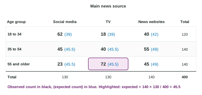
$\text{expected count} = \frac{\text{row total} \times \text{column total}}{\text{grand total}}.$

Two-way table of 400 adults by age group and main news source showing each observed count with its expected count in parentheses, for example 72 observed and 45.5 expected for adults 55 and older who use TV, found as 140 times 130 divided by 400. — **Figure 1.** Observed counts with the expected counts beside them. LevlPrep original diagram.

Worked example. Use the news poll in the figure to find two expected counts.

18 to 34, news websites: $\frac{120 \times 140}{400} = 42$ . The observed count is 40, close to it.

55 and older, TV: $\frac{140 \times 130}{400} = 45.5$ . The observed count is 72, far above it: older adults use TV more than "no association" predicts.

Expected counts need not be whole numbers, and you should not round them. In each row they add up to the row total, and in each column to the column total.

The chi-square statistic

To measure how far the whole table is from $H_0$ , compare every observed count $O$ with its expected count $E$ :

$\chi^2 = \sum \frac{(O - E)^2}{E}.$

Squaring makes every gap count, whether the observed count is above or below; dividing by $E$ puts gaps on a fair scale, since a gap of 10 matters more when 20 were expected than when 200 were. If the table matched $H_0$ exactly, $\chi^2$ would be 0. The farther the observed counts sit from the expected counts, the larger $\chi^2$ gets, and the stronger the evidence against $H_0$ . The next topic shows how large is large.

Conditions

Random: one random sample (independence), or separate random samples or random assignment (homogeneity), in the words of the problem.
10%: when sampling without replacement, each sample is less than 10% of its population.
Large counts: every expected count is at least 5. Not the observed counts, and not 10.

In the news poll, the smallest expected count is 39, so the condition is met easily. If one expected count were 3.2, a chi-square test would not be reliable, no matter how large the other cells are.

Writing it up

For the news poll: a chi-square test for independence. $H_0$ : there is no association between age group and main news source among adults in the city. $H_a$ : there is an association between age group and main news source among adults in the city. Random: a random sample of 400 adults. 10%: 400 is less than 10% of the city's adults. Large counts: every expected count is at least 39, so at least 5.