Carrying Out a Two-Proportion Test — AP® Statistics Notes

With the setup done, carrying out a two-sample z test takes three more moves: compute the test statistic, find the p-value, and write the conclusion. Each move follows from one idea: we act as if the null hypothesis were true and ask how surprising the data would be.

The test statistic

Every standardized test statistic in this course has the same form:

$\dfrac{\text{statistic} - \text{null value}}{\text{standard error of the statistic}}$

For two proportions the statistic is $\hat{p}_1 - \hat{p}_2$ and the null value is 0. If $H_0$ is true, both groups share one proportion, estimated by $p_c$ , so the standard error uses $p_c$ for both groups:

$z = \frac{(\hat{p}_1 - \hat{p}_2) - 0}{\sqrt{p_c(1 - p_c)\left(\frac{1}{n_1} + \frac{1}{n_2}\right)}}.$

The denominator is the same as $\sqrt{\frac{p_c(1-p_c)}{n_1} + \frac{p_c(1-p_c)}{n_2}}$ : the variances still add, but each one uses the pooled proportion. This formula is on the reference sheet.

The p-value

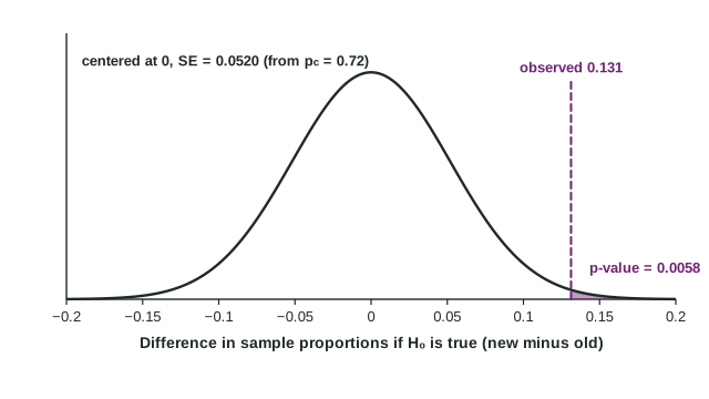
Normal curve centered at 0 with standard error 0.052, the distribution of the difference in sample proportions if the null hypothesis is true; the observed difference 0.131 is marked and the small area to its right, the p-value of about 0.006, is shaded. — **Figure 1.** The null distribution of $\hat{p}_N - \hat{p}_O$ and the shaded p-value. LevlPrep original diagram.

The p-value is the probability, assuming $H_0$ , of a difference at least as extreme as the one observed. Use the standard normal distribution and the direction of $H_a$ :

$H_a: p_1 - p_2 > 0$ : the area to the right of $z$ .
$H_a: p_1 - p_2 < 0$ : the area to the left of $z$ .
$H_a: p_1 - p_2 \ne 0$ : the area beyond $|z|$ in both tails, twice one tail.

Worked example 1 (one-sided). The city randomly assigned 160 households a new recycling bin and 140 the old bin; 125 and 91 sorted correctly. Test at $\alpha = 0.05$ whether the new bin increases correct sorting.

State. $H_0: p_N - p_O = 0$ , $H_a: p_N - p_O > 0$ , where $p_N$ and $p_O$ are the true proportions of households like these that would sort correctly with the new and the old bin.

Plan. A two-sample z test for $p_N - p_O$ . Random: the bins were randomly assigned. Large counts with $p_c = \frac{216}{300} = 0.72$ : $160(0.72) = 115.2$ , $160(0.28) = 44.8$ , $140(0.72) = 100.8$ and $140(0.28) = 39.2$ are each at least 10.

Do. $\hat{p}_N$ $= \frac{125}{160}$ $= 0.781$ and $\hat{p}_O = \frac{91}{140} = 0.650$ .

$z$ $= \frac{0.781 - 0.650}{\sqrt{0.72(0.28)\left(\frac{1}{160} + \frac{1}{140}\right)}}$ $= \frac{0.131}{0.0520}$ $= 2.53$ , and the p-value is $P(Z \ge 2.53) = 0.0058$ .

On a calculator this is a 2-proportion z test with the counts and the alternative $>$ ; it reports the same $z$ and p-value.

Conclude. Because the p-value of 0.0058 is less than $\alpha = 0.05$ , we reject $H_0$ . There is convincing evidence that the true proportion of households like these that sort their recycling correctly is greater with the new bin than with the old bin. Because the bins were randomly assigned, the new bin can be credited with the improvement, for households like these volunteers.

The figure shows why the p-value is so small: if the bin made no difference, a gap of 0.131 would be more than 2.5 standard errors from 0.

Worked example 2 (two-sided). Independent random samples of 150 residents find 45 in Lakeview and 63 in Hillcrest who take transit to work. Is there convincing evidence that the true proportions differ, at $\alpha = 0.05$ ?

$p_c$ $= \frac{45 + 63}{300}$ $= 0.36$ ; $\hat{p}_L = 0.30$ and $\hat{p}_H = 0.42$ .

$z$ $= \frac{0.30 - 0.42}{\sqrt{0.36(0.64)\left(\frac{1}{150} + \frac{1}{150}\right)}}$ $= \frac{-0.12}{0.0554}$ $= -2.17$ , and the p-value is $2P(Z \le -2.17) = 0.030$ .

Because 0.030 is less than 0.05, we reject $H_0$ . There is convincing evidence that the true proportion of residents who take transit to work is different in Lakeview and Hillcrest.

Reading a p-value and a conclusion

Interpret a p-value with its condition first: "Assuming the true proportions are equal, there is a 0.0058 probability of getting a difference in sample proportions of 0.131 or more by chance." It is never the probability that $H_0$ is true.

When the p-value is large, say "fail to reject $H_0$ " and "there is not convincing evidence that ...". Never write "accept $H_0$ " or "the proportions are the same": the data are consistent with no difference, but a real difference may be too small for these samples to detect.

Errors and scope

Decision	Possible error	In the recycling study
Reject $H_0$	Type I	concluding the new bin helps when it truly makes no difference
Fail to reject $H_0$	Type II	missing a real improvement from the new bin

Random assignment allows a cause-and-effect conclusion; random samples allow generalizing to the populations sampled. A study needs the matching design for each kind of conclusion. A voluntary response sample, such as people who choose to vote on a website, supports neither, however small its p-value.