Sampling Distribution of a Mean — AP® Statistics Notes

Unit 3 asked how a sample proportion $\hat{p}$ varies from sample to sample. Unit 4 asks the same question about a sample mean $\bar{x}$ . Every inference procedure for means in this unit rests on the answer, so it is worth getting exactly right: the center, the spread and the shape of the sampling distribution of $\bar{x}$ .

A population, and many samples from it

A coffee chain records the wait time of every car at its drive-through (invented data). Over thousands of cars, the mean wait is $\mu = 4.2$ minutes and the standard deviation is $\sigma = 2.8$ minutes. Most cars wait 2 or 3 minutes; a few wait 10 or more, so the distribution is strongly skewed right.

A manager takes a random sample of cars and computes the mean wait $\bar{x}$ . A second random sample gives a different $\bar{x}$ , a third another. If you could take every possible sample of the same size and plot all the means, you would have the sampling distribution of $\bar{x}$ . The figure shows 5,000 simulated sample means for samples of 4 cars and of 40 cars.

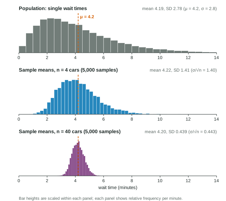
Figure 1. The population of wait times, then 5,000 simulated sample means for n = 4 and n = 40. Same center, smaller spread, more normal shape. LevlPrep original diagram.

Three things stand out in the figure. The means pile up around 4.2 minutes. They spread out much less than single wait times. And with 40 cars, the skew is gone: the means form a bell shape.

Center: the sample mean is unbiased

Some samples happen to catch more slow cars, some fewer. Over all possible samples, the overestimates and underestimates balance exactly. So the mean of the sampling distribution equals the population mean:

$\mu_{\bar{x}} = \mu.$

This holds for every sample size and every population shape. In the language of Unit 3, $\bar{x}$ is an unbiased estimator of $\mu$ .

Spread: divide by the square root of n

Why do means vary less than single values? A mean adds $n$ values and divides by $n$ . A slow car in the sample is usually offset, at least partly, by quick ones. The more cars you average, the more the high and low values cancel. The exact result, for independent observations, is

$\sigma_{\bar{x}} = \frac{\sigma}{\sqrt{n}}.$

This is the standard deviation of the sample mean. Notice the square root. To cut the spread in half, you need four times as many observations, because $\sqrt{4} = 2$ . Going from 16 bags to 64 bags halves the spread; it does not quarter it.

The formula needs independent observations. Sampling without replacement makes the draws slightly dependent, so check the 10% condition: the sample is less than 10% of the population. A sample of 40 cars from thousands passes easily. A sample of 60 apartments from a complex of 400 does not ( $60 > 40$ ), and then $\frac{\sigma}{\sqrt{n}}$ overstates the true spread.

Worked example 1. For random samples of 40 cars, find the mean and standard deviation of the sampling distribution of $\bar{x}$ .

Center: $\mu_{\bar{x}} = \mu = 4.2$ minutes.

Spread: $\sigma_{\bar{x}}$ $= \frac{\sigma}{\sqrt{n}}$ $= \frac{2.8}{\sqrt{40}}$ $= 0.443$ minutes.

The 10% condition holds: 40 cars is less than 10% of the thousands of cars served last month.

Shape: normal population, or a large sample

The shape depends on the population and on $n$ .

Population	Sample size	Shape of the sampling distribution of $\bar{x}$
Normal	any $n$	Normal
Not normal, or unknown	$n \ge 30$	Approximately normal (central limit theorem)
Skewed	small $n$	Skewed the same way as the population, less strongly

The central limit theorem (Unit 2) is the reason the second row works: averaging enough values smooths away skew. A common rule of thumb is $n \ge 30$ ; a very strongly skewed population may need more.

Be careful what the theorem says. It is about the distribution of many sample means. It does not say the 40 wait times in one sample look normal. A random sample looks like its population, so a sample of wait times is skewed right too.

Probabilities about a sample mean

Once the sampling distribution is approximately normal, standardize with the standard deviation of $\bar{x}$ , not of single values:

$z = \frac{\bar{x} - \mu}{\sigma/\sqrt{n}}.$

Worked example 2. What is the probability that the mean wait of a random sample of 40 cars is more than 5 minutes?

Shape: $n = 40 \ge 30$ , so by the central limit theorem $\bar{x}$ is approximately normal, with mean 4.2 and standard deviation 0.443 (worked example 1).

Expression and substitution: $z$ $= \frac{\bar{x} - \mu}{\sigma/\sqrt{n}}$ $= \frac{5 - 4.2}{2.8/\sqrt{40}}$ $= 1.81$ .

Answer: $P(\bar{x} > 5)$ $= P(z > 1.81)$ $= 0.035$ . Technology gives the same with a normal distribution of mean 4.2 and standard deviation 0.443, area above 5. A sample mean above 5 minutes would happen in only about 3.5% of samples, so it would be surprising if the true mean were really 4.2.

Compare one car. $P(\text{one wait} > 5)$ cannot be found with a normal model at all, because single wait times are skewed. Even for a normal population, one value is far more likely to land far from $\mu$ than a mean is. For phone batteries with mean 12.5 hours and standard deviation 1.6 hours (normal), one battery lasts more than 13 hours with probability $P\left(z > \frac{13 - 12.5}{1.6}\right)$ $= P(z > 0.31)$ $= 0.38$ , but the mean of 10 batteries does so with probability only $P\left(z > \frac{13 - 12.5}{1.6/\sqrt{10}}\right)$ $= P(z > 0.99)$ $= 0.16$ .

What to remember

Center: $\mu_{\bar{x}} = \mu$ .
Spread: $\sigma_{\bar{x}} = \frac{\sigma}{\sqrt{n}}$ , after checking the 10% condition.
Shape: normal if the population is normal; approximately normal if $n \ge 30$ ; otherwise it keeps some skew.
Always say which condition gives the normal shape, in words, with the numbers: "the population is normal" or " $n = 40 \ge 30$ , so the central limit theorem applies".

In real studies, $\sigma$ is almost never known. The next topic replaces it with the sample standard deviation $s$ and shows the price of doing so.