Unit 4 · Topic 4.1 Beta

Sampling Distributions for Sample Means

The sample mean x-bar has a sampling distribution centered at μ with standard deviation (σ)/(√n) (10% condition).

Practice 3: Analyze DataPractice 4: Interpret Results

Part 1 · Hook

Why this matters

A coffee chain times every car at its drive-through. Most cars wait 2 or 3 minutes, a few wait 12. If a manager averages a random sample of 40 cars, how far can that average land from the true mean of 4.2 minutes? The answer is a whole distribution, and it is much narrower and much more normal than the wait times themselves.

Part 2 · Before you start

What this builds on

Part 3 · Prerequisite check

Quick check before you start

1. A sampling distribution shows

the values of a statistic over many random samples of the same size
the values in one sample
the values in the whole population
the sample sizes a study could use

Show the answer

A sampling distribution is the distribution of a statistic, such as $\bar{x}$ , across all possible samples of one size.

Correct: the values of a statistic over many random samples of the same size:
the values in one sample:
the values in the whole population:
the sample sizes a study could use:

2. Heights are normal with mean 170 cm and standard deviation 8 cm. What is the z-score of 182 cm?

1.5
12
0.67
-1.5

Show the answer

$z = \frac{182 - 170}{8} = 1.5$ : the value minus the mean, over the standard deviation.

Correct: 1.5:
12:
0.67:
-1.5:

3. Why does the 10% condition matter when sampling without replacement?

It keeps the observations close enough to independent for the standard deviation formula
It makes the sampling distribution normal
It removes bias from the sample
It makes the sample size large enough

Show the answer

Drawing a small share of a large population barely changes what is left, so the draws act independent.

Correct: It keeps the observations close enough to independent for the standard deviation formula:
It makes the sampling distribution normal:
It removes bias from the sample:
It makes the sample size large enough:

Part 4 · See it

See it first

Left: the skewed population of wait times. Middle and right: 5,000 simulated sample means for samples of 4 and of 40 cars. The center stays at 4.2 minutes, the spread shrinks like

\frac{\sigma}{\sqrt{n}}

, and the shape becomes normal. LevlPrep original diagram.

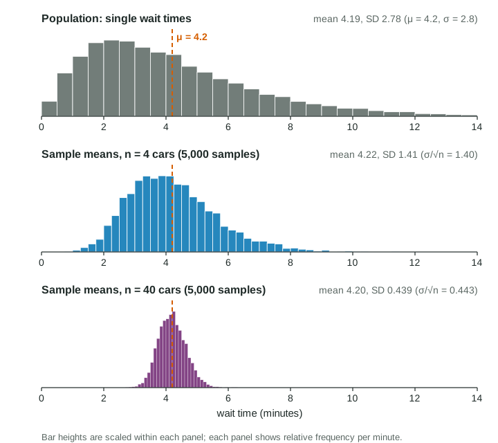
Part 5 · Step by step

How it works, step by step

Each sample mean averages $n$ valueshigh and low values partly cancel, so means vary less than single values
On average over many samples, $\bar{x}$ hits the population mean $\mu_{\bar{x}} = \mu$ : the sample mean is unbiased
The variance of an average of $n$ independent values is $\frac{\sigma^2}{n}$ the standard deviation of $\bar{x}$ is $\sigma_{\bar{x}} = \frac{\sigma}{\sqrt{n}}$ (when the sample is under 10% of the population)
Averaging many values smooths away skewfor $n \ge 30$ the sampling distribution is approximately normal (the central limit theorem); for a normal population it is normal at any $n$
With a normal model, center and spreada z-score $\frac{\bar{x} - \mu}{\sigma/\sqrt{n}}$ gives probabilities about sample means

Part 6 · Key ideas

Key ideas

Center: $\mu_{\bar{x}} = \mu$ for every sample size.
Spread: $\sigma_{\bar{x}} = \frac{\sigma}{\sqrt{n}}$ , valid when the sample is less than 10% of the population. Four times the sample size halves the spread.
Shape: normal if the population is normal; approximately normal if $n \ge 30$ (central limit theorem); otherwise it keeps some of the population's skew.
The central limit theorem is about the distribution of many sample means, not about the data in one sample.

Part 7 · Misconception

A common mistake

The wrong idea: With a large sample, the data become normal, so a skewed population gives a normal sample.

What actually happens: A large random sample looks like the population, skew and all. What becomes approximately normal is the sampling distribution of $\bar{x}$ , the pattern of the means over many samples.

Part 8 · Check yourself

Check yourself

Exam-style questions. Anything you miss goes into your review queue.

Table

Drive-through wait times

A coffee chain records the wait time of every car at its drive-through windows (invented data). Over many thousands of cars, the wait times have mean $\mu = 4.2$ minutes and standard deviation $\sigma = 2.8$ minutes, and their distribution is strongly skewed right. A manager takes a random sample of 40 cars from last month and computes the sample mean wait time $\bar{x}$ .

The population of wait times and the sample
Quantity	Value
Population mean	4.2 minutes
Population standard deviation	2.8 minutes
Population shape	strongly skewed right
Sample size	40 cars, chosen at random

1. What are the mean and the standard deviation of the sampling distribution of $\bar{x}$ for samples of 40 cars?

Mean 4.2 minutes, standard deviation about 0.44 minutes
Mean 4.2 minutes, standard deviation 2.8 minutes
Mean 4.2 minutes, standard deviation 0.07 minutes
Mean 0.44 minutes, standard deviation 2.8 minutes

Show the answer

$\mu_{\bar{x}} = \mu = 4.2$ minutes and $\sigma_{\bar{x}}$ $= \frac{\sigma}{\sqrt{n}}$ $= \frac{2.8}{\sqrt{40}}$ $= 0.443$ minutes.

Correct: Mean 4.2 minutes, standard deviation about 0.44 minutes: The mean of $\bar{x}$ equals $\mu = 4.2$ , and its standard deviation is $\frac{2.8}{\sqrt{40}} \approx 0.44$ minutes.
Mean 4.2 minutes, standard deviation 2.8 minutes: 2.8 minutes is the spread of single wait times. Averages of 40 cars vary much less: divide by $\sqrt{40}$ .
Mean 4.2 minutes, standard deviation 0.07 minutes: That divides 2.8 by 40. The standard deviation of $\bar{x}$ divides by the square root of $n$ , not by $n$ .
Mean 0.44 minutes, standard deviation 2.8 minutes: The center does not shrink. The sample mean is an unbiased estimator, so its mean is $\mu = 4.2$ .

2. The wait times are strongly skewed. Why is a normal model still reasonable for the sampling distribution of $\bar{x}$ ?

The population of wait times is approximately normal
40 cars is less than 10% of the cars served
The sample size of 40 is at least 30, so the central limit theorem applies
The cars were chosen at random from last month

Show the answer

The central limit theorem: for a random sample with $n \ge 30$ , the sampling distribution of $\bar{x}$ is approximately normal even when the population is skewed.

The population of wait times is approximately normal: The stimulus says the population is strongly skewed right. The normal shape comes from the large sample, not the population.
40 cars is less than 10% of the cars served: The 10% condition justifies the standard deviation formula. It says nothing about shape.
Correct: The sample size of 40 is at least 30, so the central limit theorem applies: With $n = 40 \ge 30$ , the central limit theorem says the sampling distribution of $\bar{x}$ is approximately normal whatever the population shape.
The cars were chosen at random from last month: Random selection is needed, but it does not by itself make the shape normal. The sample size does that.

3. Write the expression for the z-score of a sample mean of 5 minutes in the sampling distribution of $\bar{x}$ . Type it as you would on the exam, for example (a - b)/(c/sqrt(n)).

Type the expression as on the exam, with the values substituted.

Show the answer

$z$ $= \frac{\bar{x} - \mu}{\sigma/\sqrt{n}}$ $= \frac{5 - 4.2}{2.8/\sqrt{40}}$ $= 1.81$ . The standard deviation in the denominator is the one for $\bar{x}$ , not for single cars.

Answer: $\frac{5 - 4.2}{\frac{2.8}{\sqrt{40}}}$

4. What is the probability that the mean wait time of the 40 sampled cars is more than 5 minutes?

Type a number. A table answer and a calculator answer are both accepted.

Show the answer

The sampling distribution of $\bar{x}$ is approximately normal with mean 4.2 and standard deviation $\frac{2.8}{\sqrt{40}} = 0.443$ . $P(\bar{x} > 5)$ $= P\left(z > \frac{5 - 4.2}{0.443}\right)$ $= P(z > 1.81)$ $= 0.035$ .

Answer: 0.0354

5. A random sample of 50 is taken from a large, strongly skewed population with mean $\mu$ and standard deviation $\sigma$ . Which statements are true? Select all that apply.

The sampling distribution of $\bar{x}$ has mean $\mu$
The sampling distribution of $\bar{x}$ has standard deviation $\frac{\sigma}{\sqrt{50}}$
The sampling distribution of $\bar{x}$ is approximately normal
The 50 values in the sample are approximately normal
The standard deviation of $\bar{x}$ is $\sigma$
The sampling distribution of $\bar{x}$ is skewed right, like the population

Show the answer

Center $\mu$ , spread $\frac{\sigma}{\sqrt{n}}$ and an approximately normal shape describe the sampling distribution of $\bar{x}$ , not the sample itself.

Correct: The sampling distribution of $\bar{x}$ has mean $\mu$ : Right: $\bar{x}$ is unbiased for $\mu$ .
Correct: The sampling distribution of $\bar{x}$ has standard deviation $\frac{\sigma}{\sqrt{50}}$ : Right: the population is large, so the 10% condition holds.
Correct: The sampling distribution of $\bar{x}$ is approximately normal: Right: $n = 50 \ge 30$ , so the central limit theorem applies.
The 50 values in the sample are approximately normal: The sample looks like the population, so it is skewed too. The central limit theorem is about the means of many samples.
The standard deviation of $\bar{x}$ is $\sigma$ : Averages vary less than single values; divide $\sigma$ by $\sqrt{50}$ .
The sampling distribution of $\bar{x}$ is skewed right, like the population: With 50 values in each mean, the skew is smoothed away; the central limit theorem gives an approximately normal shape.

6. For the batteries above (mean 12.5 hours, standard deviation 1.6 hours, normal), which is more likely: one battery lasting more than 13 hours, or the mean of 10 batteries being more than 13 hours?

The mean of 10 batteries being more than 13 hours
One battery lasting more than 13 hours
They are equally likely, since both have mean 12.5
It depends on whether 10 is at least 30

Show the answer

One battery: $z$ $= \frac{13 - 12.5}{1.6}$ $= 0.31$ , probability 0.38. A mean of 10: $z$ $= \frac{13 - 12.5}{0.506}$ $= 0.99$ , probability 0.16.

The mean of 10 batteries being more than 13 hours: A mean of 10 stays closer to 12.5, so going past 13 is less likely for the mean.
Correct: One battery lasting more than 13 hours: Single batteries vary more, so a value 0.5 hours above the mean is less unusual for one battery (about 0.38) than for a mean of 10 (about 0.16).
They are equally likely, since both have mean 12.5: The centers match, but the spreads differ, and spread decides how likely 13 is.
It depends on whether 10 is at least 30: The population is normal, so the sampling distribution is normal; the comparison is about spread.

Part 9 · Summary

Summary

The sample mean

\bar{x}

has a sampling distribution centered at

\mu

with standard deviation

\frac{\sigma}{\sqrt{n}}

(10% condition). It is normal for a normal population and approximately normal for

n \ge 30

by the central limit theorem. Standardize with

z = \frac{\bar{x} - \mu}{\sigma/\sqrt{n}}

to find probabilities about a sample mean.

Part 10 · Up next

What comes next

Part 11 · Connections

Connections

Question set for this topic