Constructing a Confidence Interval for a Population Mean or Population Mean Difference
When σ is unknown, a confidence interval for a mean is x-bar ± t*s/(√n) with t* from the t distribution with n − 1 degrees of freedom.
Part 1 · Hook
Why this matters
Part 2 · Before you start
What this builds on
Part 3 · Prerequisite check
Quick check before you start
1. A confidence interval has the form
- statistic (critical value)(standard error)
- statistic standard error
- parameter margin of error
- critical value statistic
Show the answer
Point estimate plus or minus the margin of error, and the margin of error is the critical value times the standard error.
- Correct: statistic (critical value)(standard error):
- statistic standard error:
- parameter margin of error:
- critical value statistic:
2. For random samples of size (under 10% of the population), the standard deviation of is
Show the answer
Means vary less than single values, by a factor of .
- Correct: :
- :
- :
- :
3. In a matched pairs design,
- each subject (or pair of similar subjects) gets both treatments
- subjects are split into two unrelated groups
- no treatment is imposed
- every subject gets a placebo
Show the answer
Matched pairs compare two treatments within each pair, so the two responses belong together.
- Correct: each subject (or pair of similar subjects) gets both treatments:
- subjects are split into two unrelated groups:
- no treatment is imposed:
- every subject gets a placebo:
Part 4 · See it
See it first
Part 5 · Step by step
How it works, step by step
- The population standard deviation is unknownestimate it with the sample standard deviation , so the standard error is
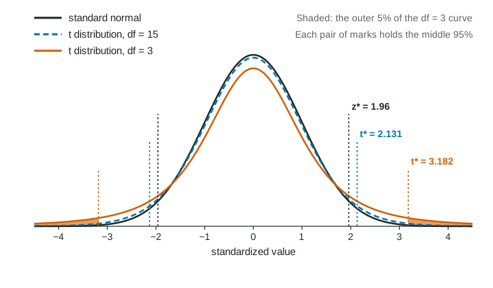
- itself varies from sample to sample varies more than a z-score: it follows a t distribution with degrees of freedom
- The t distribution has heavier tails than the normalthe critical value is larger than , more so for small samples
- Put it togetherthe one-sample t interval is
- For paired data, subtract within each pair firstthe same interval on the differences, , estimates the mean difference
Part 6 · Key ideas
Key ideas
- One-sample t interval: , with from the t distribution with .
- Conditions: random sample (or random assignment); 10% condition when sampling without replacement; normal/large sample (population normal, or , or a graph of the sample with no strong skew or outliers).
- Paired data (two measurements on the same individual or matched pair): work with the differences, one sample, parameter .
- Interpretation: "We are 95% confident that the interval from ... to ... captures the true mean ..."
Part 7 · Misconception
A common mistake
The wrong idea: With a sample of 30 or more, use for a mean.
What actually happens: Whenever stands in for an unknown , use with degrees of freedom. For large samples is close to , but it is still the right value to use.
Part 8 · Check yourself
Check yourself
Exam-style questions. Anything you miss goes into your review queue.
Graph
One-way distances of 25 bike commuters
A city transportation office surveyed a random sample of 25 of the city's many thousands of bike commuters and recorded each one's one-way commute distance (invented data). The sample mean is miles and the sample standard deviation is miles.
1. What is the critical value for a 95% confidence interval for the mean distance?
Type a number. A table answer and a calculator answer are both accepted.
Show the answer
With , the middle 95% of the t distribution lies between and , so (Table B, df 24, 95% column, or technology: the 0.975 quantile of t with 24 df).
- Answer: 2.064
2. Write the expression for the 95% confidence interval for the mean one-way distance, with . Type it as on the exam, for example a +/- b*c/sqrt(n).
Type the expression as on the exam, with the values substituted.
Show the answer
- Answer:
3. Construct the 95% confidence interval for the mean one-way distance of the city's bike commuters, in miles.
Type the interval as "from a to b".
Show the answer
- Answer: from 5.6 to 8
4. The sample has only 25 commuters. How is the normal/large sample condition met?
- 25 is less than 10% of the many thousands of bike commuters in the city
- The dotplot of the sample shows no strong skew and no outliers
- The sample was chosen at random
- 25 is at least 10
Show the answer
Normal/large sample: the population is normal, or , or (as here) a graph of the sample shows no strong skew or outliers.
- 25 is less than 10% of the many thousands of bike commuters in the city: That is the 10% condition, about independence. It does not address the shape.
- Correct: The dotplot of the sample shows no strong skew and no outliers: With , check a graph of the sample: this dotplot is roughly symmetric with no outliers, so a t interval is reasonable.
- The sample was chosen at random: That is the random condition. The normal/large sample condition is about shape or sample size.
- 25 is at least 10: 10 is the large counts threshold for proportions. For means, either or a graph without strong skew or outliers.
5. Why does a confidence interval for a mean use instead of ?
- The data come from a skewed population
- The sample is smaller than 30
- The interval uses in place of the unknown
- By definition, intervals for means use t and intervals for proportions use z
Show the answer
With unknown, follows a t distribution with degrees of freedom, which is wider than the standard normal.
- The data come from a skewed population: The shape condition is separate. Even for a normal population, using calls for t.
- The sample is smaller than 30: Large samples use too, whenever is estimated by .
- Correct: The interval uses in place of the unknown : Replacing with adds variability, because changes from sample to sample. The t distribution, with heavier tails, accounts for it.
- By definition, intervals for means use t and intervals for proportions use z: There is a reason: for means the standard error estimates with , which adds extra uncertainty.
6. The 95% confidence interval for the mean one-way distance of the city's bike commuters is from 5.60 to 8.00 miles. Build the interpretation.
Write the conclusion in context.
Show the answer
The confidence is about the method capturing the parameter, the true mean distance of all the city's bike commuters, not about individual commuters or the sample mean.
- A full-credit answer: We are 95% confident that the interval from 5.60 to 8.00 miles captures the true mean one-way distance of all the city's bike commuters.
7. A researcher records the ages of both partners in a random sample of 30 married couples and wants to estimate how much older husbands are than wives, on average. Which procedure fits?
- Two separate t intervals, one for the husbands' ages and one for the wives' ages, then compare
- A two-sample z interval for the difference of two proportions
- A one-sample z interval using 1.96
- A one-sample t interval for the mean of the 30 differences, husband minus wife
Show the answer
Pairs: compute husband minus wife for each couple, then with 29 df.
- Two separate t intervals, one for the husbands' ages and one for the wives' ages, then compare: Two intervals do not estimate the mean of the paired difference, and they ignore the pairing.
- A two-sample z interval for the difference of two proportions: Ages are quantitative, so this is about means, not proportions.
- A one-sample z interval using 1.96: The population standard deviation of the differences is unknown, so use .
- Correct: A one-sample t interval for the mean of the 30 differences, husband minus wife: The two ages in a couple belong together, so the data are paired: one difference per couple, then a t interval for .
Part 9 · Summary
Summary
Part 10 · Up next
What comes next
Part 11 · Connections