Interval for a Mean — AP® Statistics Notes

In Unit 3 you built confidence intervals for a proportion. The recipe for a mean has the same shape, statistic plus or minus a margin of error, with one change that matters: you almost never know the population standard deviation, so you estimate it, and that calls for a new critical value.

The problem with sigma

The last topic gave the standard deviation of $\bar{x}$ as $\frac{\sigma}{\sqrt{n}}$ . But if you do not know the population mean $\mu$ (that is why you are estimating it), you almost surely do not know $\sigma$ either. The natural fix is to use the sample standard deviation $s$ . The estimated standard deviation of $\bar{x}$ is its standard error:

$\text{SE} = \frac{s}{\sqrt{n}}.$

Here is the catch. $s$ changes from sample to sample. Some samples happen to have a small $s$ , which makes the standardized value $\frac{\bar{x} - \mu}{s/\sqrt{n}}$ larger than a z-score would be. So this ratio does not follow the standard normal distribution. It follows a t distribution.

The t distributions

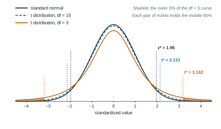
Three bell-shaped density curves centered at 0 on an axis from -4.5 to 4.5: the standard normal (solid black), the t distribution with 15 degrees of freedom (dashed blue) and the t distribution with 3 degrees of freedom (orange), which is lowest in the middle and highest in the tails. Dashed marks show the 95% critical values: z* = 1.96, t* = 2.131 for 15 df and t* = 3.182 for 3 df. The outer 5% of the 3 df curve is shaded. — **Figure 1.** The standard normal curve and t distributions with 3 and 15 degrees of freedom, with the 95% critical values marked. LevlPrep original diagram.

A t distribution looks like the standard normal: symmetric, bell shaped, centered at 0. Its tails are heavier, because of the extra variability from $s$ . There is a different t distribution for each number of degrees of freedom. For one sample, $\text{df} = n - 1$ , the same $n - 1$ that appears in the formula for $s$ .

The more data, the better $s$ estimates $\sigma$ , and the closer the t distribution gets to the standard normal. The figure shows it: with 3 df the middle 95% reaches out to $\pm 3.182$ ; with 15 df to $\pm 2.131$ ; the standard normal stops at $\pm 1.96$ .

	z procedures (proportions)	t procedures (means)
Standard error	$\sqrt{\frac{\hat{p}(1 - \hat{p})}{n}}$	$\frac{s}{\sqrt{n}}$
Critical value	$z^*$ from the standard normal (Table A)	$t^*$ with $n - 1$ df (Table B)
Shape condition	Large counts: at least 10 successes and 10 failures	Normal/large sample: normal population, $n \ge 30$ , or no strong skew or outliers in the sample
95% critical value	1.96	depends on df: 2.262 at df 9, 2.064 at df 24, 1.984 at df 100

To read $t^*$ from Table B, find the row for your df and the column for your confidence level. If your df is not in the table (say 44), use the next smaller row (40); that is a little conservative. Technology gives the exact value: the 0.975 quantile of t with your df, for 95%.

The one-sample t interval

$\bar{x} \pm t^*\frac{s}{\sqrt{n}}, \qquad \text{df} = n - 1.$

Before you compute, check the conditions for inference, in words, with numbers:

Random: a random sample from the population, or random assignment in an experiment.
10%: when sampling without replacement, $n$ is less than 10% of the population.
Normal/large sample: the population is normal, or $n \ge 30$ (the central limit theorem), or a graph of the sample shows no strong skew and no outliers. Name the graph and what it shows.

Worked example 1. A random sample of 25 of a city's bike commuters has mean one-way distance $\bar{x} = 6.8$ miles and $s = 2.9$ miles. A dotplot of the 25 distances is roughly symmetric with no outliers. Construct a 95% confidence interval for the mean one-way distance.

Procedure: a one-sample t interval for $\mu$ , the true mean one-way distance of all the city's bike commuters.

Conditions. Random: the problem says a random sample. 10%: 25 is less than 10% of the city's many thousands of bike commuters. Normal/large sample: $n = 25 < 30$ , but the dotplot of the sample shows no strong skew and no outliers.

Expression and substitution: $\text{df} = 24$ , $t^* = 2.064$ , so $\bar{x}$ $\pm t^*\frac{s}{\sqrt{n}}$ $= 6.8$ $\pm 2.064\frac{2.9}{\sqrt{25}}$ $= 6.8$ $\pm 1.197$ .

Answer: from 5.60 to 8.00 miles.

Interpretation: We are 95% confident that the interval from 5.60 to 8.00 miles captures the true mean one-way distance of all the city's bike commuters.

The confidence level has the same meaning as in Unit 3: if we took many random samples of 25 commuters and built a 95% interval from each, about 95% of the intervals would capture the true mean distance. It does not say that 95% of commuters ride between 5.60 and 8.00 miles; the interval is about a mean, not about individual riders.

Paired data: one sample of differences

Sometimes the data come in pairs: the same student before and after a course, the left and right foot, two matched subjects in a matched pairs design. The two values in a pair belong together. They are not two independent samples. The right move is to subtract within each pair and analyze the differences as one sample. The parameter is the true mean difference, $\mu_d$ .

Worked example 2. A random sample of 10 students in a keyboarding course typed a passage on the first and last days. The differences (after minus before, in words per minute) are 8, 3, 11, 6, $-2$ , 9, 5, 7, 12, 4. Construct a 95% confidence interval for the mean change.

Summaries of the differences: $\bar{x}_d = \frac{63}{10} = 6.3$ and $s_d = 4.11$ words per minute.

Conditions. Random: a random sample of students in the course. 10%: 10 is less than 10% of all students who take it. Normal/large sample: $n = 10 < 30$ , and a dotplot of the 10 differences shows no strong skew and no outliers.

Expression and substitution: $\text{df} = 9$ , $t^* = 2.262$ , so $\bar{x}_d$ $\pm t^*\frac{s_d}{\sqrt{n}}$ $= 6.3$ $\pm 2.262\frac{4.11}{\sqrt{10}}$ $= 6.3$ $\pm 2.94$ .

Answer: from 3.36 to 9.24 words per minute.

Interpretation: We are 95% confident that the interval from 3.36 to 9.24 words per minute captures the true mean change in typing speed (after minus before) for students who take the course.

Two habits earn points here. Say which way you subtracted (after minus before), so a positive mean difference has a clear meaning. And check the shape condition on the differences, because the differences are the sample.

Common slips

Using $z^* = 1.96$ for a mean. With $s$ in the formula, use $t^*$ at every sample size.
Using $n$ instead of $n - 1$ for df.
Treating paired data as two separate samples.
Checking " $n \ge 10$ " for a mean. Ten is the large counts threshold for proportions. For means the check is normal population, $n \ge 30$ , or a graph with no strong skew or outliers.