Two-Mean Sampling Distribution — AP® Statistics Notes

The second half of Unit 4 compares two means: two orchards, two machines, two treatments in an experiment. The statistic is the difference in sample means, $\bar{x}_1 - \bar{x}_2$ . Like every statistic it varies from sample to sample, and its sampling distribution is the foundation for the intervals and tests that follow. You met the same idea for two proportions in Unit 3.

A difference of two sample means

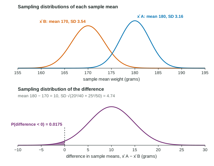
Apple weights at orchard A have mean $\mu_A = 180$ grams and standard deviation $\sigma_A = 20$ grams. At orchard B, $\mu_B = 170$ and $\sigma_B = 25$ grams (invented data). A buyer takes independent random samples, 40 apples from A and 50 from B, and computes $\bar{x}_A - \bar{x}_B$ .

From the first topic of this unit, each sample mean has its own sampling distribution:

$\bar{x}_A$ : mean 180, standard deviation $\frac{20}{\sqrt{40}} = 3.16$ grams;
$\bar{x}_B$ : mean 170, standard deviation $\frac{25}{\sqrt{50}} = 3.54$ grams.

Top: two normal curves for the sample mean apple weight, orchard A centered at 180 grams with standard deviation 3.16 and orchard B centered at 170 grams with standard deviation 3.54. Bottom: a wider normal curve for the difference of the two sample means, centered at 10 grams with standard deviation 4.74; the area below 0, shaded, is 0.0175. — **Figure 1.** The two sampling distributions, and the wider sampling distribution of their difference. LevlPrep original diagram.

Center and spread

The center is what you would guess: the difference is centered at the difference of the population means,

$\mu_{\bar{x}_1 - \bar{x}_2} = \mu_1 - \mu_2.$

The spread is where intuition often goes wrong. The means are subtracted, but the variability is not. Think about what can make $\bar{x}_A - \bar{x}_B$ come out far from 10: $\bar{x}_A$ might be unusually high, or $\bar{x}_B$ unusually low, or both. Each sample mean brings its own uncertainty, and for independent samples the uncertainties pile up. The rule is that variances add:

$\sigma_{\bar{x}_1 - \bar{x}_2} = \sqrt{\frac{\sigma_1^2}{n_1} + \frac{\sigma_2^2}{n_2}}.$

This formula is on the reference sheet. Notice its parts: each population variance is divided by its own sample size, the two are added, and then the square root is taken. Standard deviations themselves are never added, and the variances are never subtracted.

Worked example 1. Find the mean and standard deviation of the sampling distribution of $\bar{x}_A - \bar{x}_B$ .

Center: $\mu_A - \mu_B$ $= 180 - 170$ $= 10$ grams.

Spread: $\sqrt{\frac{\sigma_A^2}{n_A} + \frac{\sigma_B^2}{n_B}}$ $= \sqrt{\frac{20^2}{40} + \frac{25^2}{50}}$ $= \sqrt{10 + 12.5}$ $= 4.74$ grams.

Check: 4.74 is larger than either 3.16 or 3.54, as it should be. (Adding the standard deviations would give $3.16 + 3.54 = 6.70$ , which is too large.)

Conditions behind the formula

Independent samples: two separate random samples, or two groups formed by random assignment in an experiment. Paired data (the same runners timed twice, twins, before and after) are not independent; use the differences and the one-sample methods instead.
10% condition, for each sample: each sample is less than 10% of its own population. A sample of 60 nurses from a hospital of 450 fails it ( $60 > 45$ ) even if a second hospital is large. Random assignment in an experiment has no population to sample from, so the 10% condition does not apply there.

Shape

Populations	Sample sizes	Shape of $\bar{x}_1 - \bar{x}_2$
both normal	any	normal
not known to be normal	both $n_1 \ge 30$ and $n_2 \ge 30$	approximately normal (central limit theorem)
skewed	either sample small	not reliably normal

Each sample is checked on its own. A total of 90 apples does not help if one of the samples has only 8 from a skewed population.

Probabilities about a difference

Worked example 2. What is the probability that the buyer's sample from B comes out heavier on average than the sample from A, that is, $\bar{x}_A - \bar{x}_B < 0$ ?

Shape: $n_A = 40 \ge 30$ and $n_B = 50 \ge 30$ , so the difference is approximately normal, with mean 10 and standard deviation 4.74 grams.

Expression and substitution: $z$ $= \frac{0 - 10}{4.74}$ $= -2.11$ .

Answer: $P(\bar{x}_A - \bar{x}_B < 0)$ $= P(z < -2.11)$ $= 0.0175$ (technology; Table A gives 0.0174 for $z = -2.11$ ). Even though A's apples are heavier on average, about 2% of pairs of samples would show the opposite.

Worked example 3. Machine 1 fills bottles with mean 500.0 mL and SD 1.5 mL; machine 2 with mean 499.0 mL and SD 2.0 mL; both normal. With samples of 8 and 10 bottles, find $P(\bar{x}_1 - \bar{x}_2 > 2)$ .

Shape: both populations are normal, so the difference is normal even with small samples.

Center $500.0 - 499.0 = 1$ mL; spread $\sqrt{\frac{1.5^2}{8} + \frac{2.0^2}{10}}$ $= \sqrt{0.281 + 0.400}$ $= 0.825$ mL.

$z = \frac{2 - 1}{0.825} = 1.21$ , so $P(\bar{x}_1 - \bar{x}_2 > 2)$ $= P(z > 1.21)$ $= 0.113$ .

In practice the population standard deviations are rarely known. The next topic replaces $\sigma_1$ and $\sigma_2$ with the sample standard deviations $s_1$ and $s_2$ and builds a confidence interval for $\mu_1 - \mu_2$ .