Setting Up a Test for a Mean — AP® Statistics Notes

A significance test for a mean follows the same logic as the test for a proportion in Unit 3: assume the null hypothesis, ask how surprising the data would be, and weigh the evidence. This topic covers the first half of the job, the setup. Get it right and the calculation in the next topic is routine.

Start from the question

A delivery company advertises a mean delivery time of 30 minutes in one city. A manager suspects deliveries take longer. She takes a random sample of 45 of last month's thousands of deliveries (invented data). Three things come straight from the question, before any data are looked at:

The parameter: $\mu$ , the true mean delivery time of all the company's deliveries in the city.
The hypothesized mean $\mu_0$ : the value the null hypothesis claims, here the advertised 30 minutes.
The direction: the manager suspects longer, so the alternative is "greater than".

$H_0: \mu = 30 \qquad H_a: \mu > 30$

where $\mu$ is the true mean delivery time of all the company's deliveries in the city. This is a one-sample t test: one sample, a mean, and $\sigma$ unknown, so the t distribution with $n - 1$ degrees of freedom will measure the surprise.

The three possible alternatives match three kinds of question:

Question	Alternative
Is the mean greater than (longer, more, higher) $\mu_0$ ?	$H_a: \mu > \mu_0$
Is the mean less than (shorter, fewer, lower) $\mu_0$ ?	$H_a: \mu < \mu_0$
Is the mean different from $\mu_0$ ?	$H_a: \mu \ne \mu_0$ (two-sided)

Three rules catch most lost points. Hypotheses are about parameters: $H_0: \bar{x} = 30$ is wrong, because the sample mean is known once you have the data. The equals sign goes in $H_0$ . And the direction of $H_a$ comes from the question, never from the sample result: if the question is "different from 30" and the sample mean is 27, the alternative is still $\mu \ne 30$ .

Paired data: test the mean difference

A large gym measures the resting heart rate of a random sample of 12 members before and after a four-week breathing class (invented data). Each member gives two linked numbers, so the data are paired. As with intervals, subtract within each pair and work with the differences as one sample.

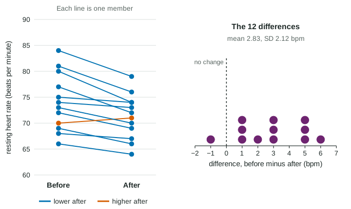
Left: a slope chart of resting heart rate for 12 gym members, before and after a breathing class, on a scale from 60 to 90 beats per minute; 11 lines slope down and one slopes up. Right: a dotplot of the 12 differences, before minus after: -1, 1, 1, 1, 2, 3, 3, 3, 5, 5, 5, 6, with mean 2.83 and standard deviation 2.12. All but one difference is above 0. — **Figure 1.** Before and after heart rates for each of the 12 members, and the dotplot of the differences. LevlPrep original diagram.

The order of subtraction sets the direction. With $d = \text{before} - \text{after}$ , a lower heart rate after the class gives a positive difference:

$H_0: \mu_d = 0 \qquad H_a: \mu_d > 0$

where $\mu_d$ is the true mean drop in resting heart rate (before minus after) for gym members who take the class. With after minus before, the same question gives $H_a: \mu_d < 0$ . Either is fine; say which one you used. This test is called a paired t test: a one-sample t test on the differences.

When are data paired? When the two values belong to the same individual (before and after, left and right) or to two individuals matched on purpose (twins, a matched pairs design). Two separate random samples, such as 20 commuters from one city and 20 from another, are not paired; Unit 4 handles them later with a different procedure.

Conditions, in words, with numbers

The conditions are the same three as for a t interval:

Random: a random sample or a randomized experiment.
10%: when sampling without replacement, $n$ is less than 10% of the population.
Normal/large sample: the population is normal, or $n \ge 30$ , or a graph of the sample (for paired data, of the differences) shows no strong skew and no outliers.

Worked example 1. Set up the delivery test.

Procedure: a one-sample t test for a mean.

Hypotheses: $H_0: \mu = 30$ , $H_a: \mu > 30$ , where $\mu$ is the true mean delivery time of all the company's deliveries in the city.

Conditions. Random: the problem says a random sample of 45 deliveries. 10%: 45 is less than 10% of last month's thousands of deliveries. Normal/large sample: $n = 45 \ge 30$ , so the central limit theorem says the sampling distribution of $\bar{x}$ is approximately normal.

Worked example 2. Set up the heart rate test.

Procedure: a paired t test for the mean difference (a one-sample t test on the differences, before minus after).

Hypotheses: $H_0: \mu_d = 0$ , $H_a: \mu_d > 0$ , where $\mu_d$ is the true mean of before minus after resting heart rate for gym members who take the class.

Conditions. Random: a random sample of 12 members who took the class. 10%: 12 is less than 10% of the members who take the class at a large gym. Normal/large sample: $n = 12 < 30$ , so look at the differences: 3, 1, 6, 1, 2, 5, $-1$ , 5, 3, 3, 5, 1. A dotplot of them shows no strong skew and no outliers.

When the condition fails, say so. A random sample of 15 commute times that is strongly skewed with one time of 95 minutes does not meet the normal/large sample condition, and a t test on it could be misleading.

Errors, set up in advance

The setup also tells you what each error would mean. For the delivery test, a Type I error would occur if the true mean delivery time of all the company's deliveries in the city is 30 minutes, but we find convincing evidence that it is greater than 30 minutes. A Type II error would occur if the true mean is greater than 30 minutes, but we do not find convincing evidence that it is. The next topic computes the evidence.