Carrying Out a Test for a Mean — AP® Statistics Notes

With the hypotheses written and the conditions checked, the rest of a t test is three steps: compute a test statistic, find its p-value, and write the conclusion. Each step has a standard form that earns the points, and a classic slip that loses them.

The t statistic

Assume the null hypothesis is true: the population mean is $\mu_0$ . Then sample means vary around $\mu_0$ , with a standard error of $\frac{s}{\sqrt{n}}$ . The question is how far the observed $\bar{x}$ is from $\mu_0$ , measured in standard errors. That is the t statistic:

$t = \frac{\bar{x} - \mu_0}{s/\sqrt{n}}, \qquad \text{df} = n - 1.$

It has the same shape as every standardized test statistic: (statistic minus null value) divided by the standard error. Because $s$ estimates $\sigma$ , the p-value comes from the t distribution, not the standard normal.

The t distribution with 44 degrees of freedom, centered at 0. A dashed line marks the observed t statistic 2.37, and the small area under the curve to its right is shaded: the one-sided p-value, 0.0112. — **Figure 1.** The t distribution with 44 df, the observed t = 2.37 and the shaded p-value. LevlPrep original diagram.

A complete test

Worked example 1. A company advertises a mean delivery time of 30 minutes. A random sample of 45 of last month's thousands of deliveries has $\bar{x} = 32.4$ minutes and $s = 6.8$ minutes (invented data). Is there convincing evidence at $\alpha = 0.05$ that the true mean is longer than 30 minutes?

State. $H_0: \mu = 30$ , $H_a: \mu > 30$ , where $\mu$ is the true mean delivery time of all the company's deliveries in the city.

Plan. One-sample t test for a mean. Random: a random sample of 45 deliveries. 10%: 45 is less than 10% of last month's deliveries. Normal/large sample: $n = 45 \ge 30$ .

Do. $t$ $= \frac{\bar{x} - \mu_0}{s/\sqrt{n}}$ $= \frac{32.4 - 30}{6.8/\sqrt{45}}$ $= \frac{2.4}{1.014}$ $= 2.37$ , with $\text{df} = 44$ . The alternative says "greater than", so the p-value is the area to the right: $P(t > 2.37) = 0.0112$ .

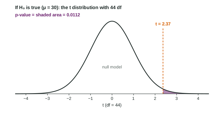
Conclude. Because the p-value of 0.0112 is less than 0.05, we reject the null hypothesis. There is convincing evidence that the true mean delivery time of all the company's deliveries in the city is greater than 30 minutes.

Technology does the "Do" step in one command, a one-sample t test from the summary statistics, and reports $t = 2.37$ , $\text{df} = 44$ , $p = 0.0112$ . On the exam, still write the formula with the numbers substituted; the calculator output alone is not work.

With Table B, find the df row (44 is not listed, so use the next smaller row, 40) and locate 2.37 between two critical values: 2.123 (one-tail probability 0.02) and 2.423 (0.01). So $0.01 < p < 0.02$ , which is enough to decide at $\alpha = 0.05$ .

Which tail?

Alternative	p-value
$H_a: \mu > \mu_0$	area to the right of $t$
$H_a: \mu < \mu_0$	area to the left of $t$
$H_a: \mu \ne \mu_0$	twice the area beyond $\|t\|$

Worked example 2 (two-sided). A random sample of 20 students at a large university slept a mean of 7.55 hours with $s = 1.09$ hours. Test $H_0: \mu = 8$ against $H_a: \mu \ne 8$ at $\alpha = 0.05$ , where $\mu$ is the true mean nightly sleep of students at the university. (Assume the conditions are met.)

$t$ $= \frac{7.55 - 8}{1.09/\sqrt{20}}$ $= -1.85$ , $\text{df} = 19$ . Two-sided: $p$ $= 2P(t < -1.85)$ $= 0.080$ .

Because the p-value of 0.080 is greater than 0.05, we fail to reject the null hypothesis. There is not convincing evidence that the true mean nightly sleep of students at the university is different from 8 hours.

Notice what the second conclusion does not say. It does not say the mean is 8 hours, and it does not say "accept $H_0$ ". The sample mean was 7.55; the data simply could not rule out 8.

Paired data: the same test on the differences

Worked example 3. For 12 randomly chosen gym members who took a breathing class, the differences in resting heart rate (before minus after) have $\bar{x}_d = 2.83$ and $s_d = 2.12$ beats per minute, with no strong skew or outliers. Test $H_0: \mu_d = 0$ against $H_a: \mu_d > 0$ at $\alpha = 0.05$ .

$t$ $= \frac{\bar{x}_d - 0}{s_d/\sqrt{n}}$ $= \frac{2.83 - 0}{2.12/\sqrt{12}}$ $= 4.62$ , $\text{df} = 11$ , $p = P(t > 4.62) = 0.0004$ .

Because the p-value of 0.0004 is less than 0.05, we reject the null hypothesis. There is convincing evidence that the true mean drop in resting heart rate (before minus after) for gym members who take the class is greater than 0.

Can the gym say the class caused the drop? No. The members were sampled at random, so the result generalizes to members who take the class, but there was no random assignment and no comparison group. Something else in those four weeks could explain it.

Interpreting the p-value

The p-value is a probability computed assuming the null hypothesis is true. For the delivery test: Assuming the true mean delivery time of all the company's deliveries is 30 minutes, there is a 0.0112 probability of getting a sample mean of 32.4 minutes or more by chance in a random sample of 45 deliveries.

It is not the probability that $H_0$ is true, and it is not the probability that the result is due to chance. Small p-values say the data would be surprising if $H_0$ were true, and that is the evidence for $H_a$ .