Setting Up a Two-Sample t Test — AP® Statistics Notes

The test for a difference of two means asks the same kind of question as the interval: is there convincing evidence that two true means differ, or that one is larger? Before the arithmetic comes the setup, and with two groups there is one new decision to make first: are the data paired, or are they two independent groups?

Paired or two independent groups?

The design decides, not the numbers. Look at how the data were produced.

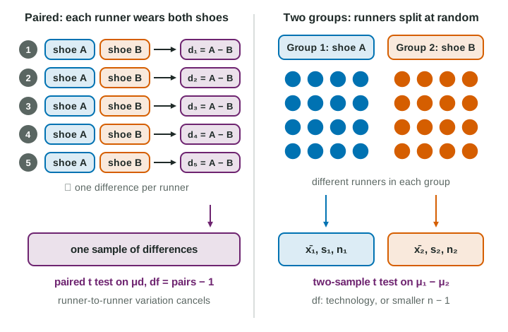
Left panel, paired design: five numbered runners each run in shoe A and in shoe B, and each gives one difference, A minus B; the differences form one sample, analyzed with a paired t test on the mean difference with df equal to the number of pairs minus 1. Right panel, two groups: runners are split at random into group 1 wearing shoe A and group 2 wearing shoe B, different runners in each; each group gives its own mean, standard deviation and size, analyzed with a two-sample t test on mu 1 minus mu 2, with technology df or the smaller n minus 1. — **Figure 1.** Paired designs give one list of differences; two-sample designs give two independent groups. LevlPrep original diagram.

	Paired	Two independent groups
How the data arise	each unit measured twice, or units matched in pairs	two separate random samples, or random assignment to two groups
Examples	before and after; both shoes on the same runner; twins	brand X phones and brand Y phones; runners split into two shoe groups
Parameter	$\mu_d$ , the true mean difference	$\mu_1 - \mu_2$ , the difference of true means
Test	paired t test (one-sample t on the differences)	two-sample t test
df	$n - 1$ , where $n$ is the number of pairs	technology, or the smaller of $n_1 - 1$ and $n_2 - 1$

A coach with 40 runners and two shoe designs can do either. In plan 1, every runner runs once in each shoe, in random order: paired. In plan 2, the runners are randomly split 20 and 20: two groups. Plan 1 is usually better at detecting a small effect. Runners differ from each other by minutes; a shoe might change a time by seconds. Pairing compares each runner with themselves, so the large runner-to-runner variation drops out of the differences.

Hypotheses for two means

For two independent groups, the null hypothesis says the true means are equal, and the alternative comes from the question:

$H_0: \mu_1 - \mu_2 = 0 \qquad H_a: \mu_1 - \mu_2 > 0, \quad < 0, \quad \text{or} \ne 0.$

You may also write $H_0: \mu_1 = \mu_2$ and $H_a: \mu_1 > \mu_2$ . Either way, define both parameters in context, and keep the order of subtraction consistent from the hypotheses to the conclusion.

Worked example 1. A consumer group buys a random sample of 15 brand X phones and an independent random sample of 15 brand Y phones and runs each until the battery dies while streaming (invented data). Does brand X last longer on average? Set up the test.

Procedure: a two-sample t test for $\mu_X - \mu_Y$ .

Hypotheses: $H_0: \mu_X - \mu_Y = 0$ , $H_a: \mu_X - \mu_Y > 0$ , where $\mu_X$ is the true mean battery life while streaming of all new brand X phones and $\mu_Y$ the same for brand Y.

Conditions. Random: independent random samples of each brand. 10%: 15 is less than 10% of all phones sold, for each brand. Normal/large sample: both samples have $n = 15 < 30$ , but boxplots of both show no strong skew and no outliers.

Worked example 2. For plan 2 of the shoe study (runners randomly assigned 20 to shoe A, 20 to shoe B), the coach asks whether the mean 5 km time differs between the shoes.

Hypotheses: $H_0: \mu_A - \mu_B = 0$ , $H_a: \mu_A - \mu_B \ne 0$ , where $\mu_A$ and $\mu_B$ are the true mean 5 km times in shoes A and B for runners like these. "Differs" means two-sided.

Conditions. Random: random assignment of runners to shoes. 10%: not needed, since this is an experiment, not a sample from a population. Normal/large sample: 20 per group, so check that a graph of each group's times shows no strong skew or outliers.

Conditions, group by group

Every condition is checked for each group. A sample of 40 delivery times from company P passes the normal/large sample condition by size, but if the sample of 12 from company Q is strongly skewed with an outlier, the test is not appropriate: P passing does not rescue Q. Different sample sizes are fine, and the two standard deviations do not need to match; the test uses each one separately.

When it is a one-sample test after all

If one of the two means is a known standard rather than a second sample (an old bulb's long-established mean life of 1,200 hours, say), there is only one sample: test $H_0: \mu = 1200$ with a one-sample t test. A two-sample test is for two groups that both carry sampling variability.

Errors in context

For the battery test, a Type I error would occur if the two brands have the same true mean battery life but we find convincing evidence that brand X's is greater. A Type II error would occur if the true mean battery life of brand X phones is greater than that of brand Y phones, but we do not find convincing evidence that it is greater. The next topic computes the test statistic and the p-value.