Interval for Two Means — AP® Statistics Notes

The last topic described how $\bar{x}_1 - \bar{x}_2$ varies when the population standard deviations are known. In practice they are not, so, exactly as for one mean, we estimate them with the sample standard deviations and switch from $z^*$ to $t^*$ . The result is the two-sample t interval.

The interval

Replace $\sigma_1$ and $\sigma_2$ with $s_1$ and $s_2$ in the standard deviation of $\bar{x}_1 - \bar{x}_2$ . That gives the standard error

$\text{SE} = \sqrt{\frac{s_1^2}{n_1} + \frac{s_2^2}{n_2}},$

and the interval has the familiar form, statistic plus or minus critical value times standard error:

$(\bar{x}_1 - \bar{x}_2) \pm t^*\sqrt{\frac{s_1^2}{n_1} + \frac{s_2^2}{n_2}}.$

The parameter is $\mu_1 - \mu_2$ , the difference in true means. Always say which group is "1": the order of subtraction decides the sign of every value in the interval. Reversing the order flips the interval: from 2.1 to 6.5 for $\mu_A - \mu_B$ becomes from $-6.5$ to $-2.1$ for $\mu_B - \mu_A$ .

Degrees of freedom: two accepted choices

For two samples, the t distribution that fits is only approximate, and its degrees of freedom come from a long formula (the Welch formula) that technology computes for you. It is usually not a whole number. If you are using Table B instead, the safe choice is the conservative degrees of freedom, the smaller of $n_1 - 1$ and $n_2 - 1$ .

Choice	Spaced versus massed example	Effect
Technology (Welch) df	df = 25.6, $t^* = 2.057$	the more accurate interval
Conservative df, smaller $n - 1$	df = 13, $t^* = 2.160$	slightly wider: at least the stated confidence

Both are accepted on the exam. Say which you used.

Conditions, for each group

Random: two independent random samples, or two groups formed by random assignment in an experiment.
10%: when sampling without replacement, each sample is less than 10% of its own population. (Not needed for random assignment.)
Normal/large sample: for each group, the population is normal, or $n \ge 30$ , or a graph of that group's data shows no strong skew and no outliers.

Independence between the groups matters too. If the same people are measured twice, or the units come in matched pairs, the data are paired: use the differences and a one-sample t interval instead.

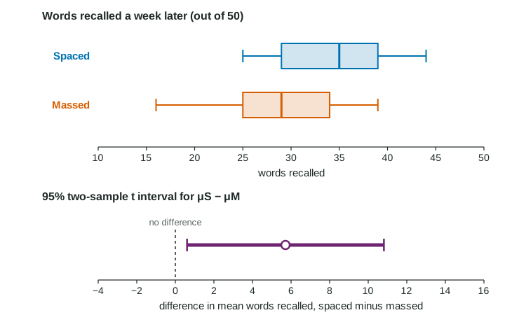
Top: side-by-side boxplots of words recalled. Spaced practice: min 25, Q1 29, median 35, Q3 39, max 44. Massed practice: min 16, Q1 25, median 29, Q3 34, max 39. Neither has outliers. Bottom: the 95% confidence interval for the true difference in mean recall, spaced minus massed, from 0.61 to 10.81 words, centered at 5.71, entirely to the right of a dashed line at 0. — **Figure 1.** Words recalled by the two groups, and the 95% interval for the difference in true means. LevlPrep original diagram.

Worked example 1 (an experiment). Twenty-eight volunteers were randomly assigned, 14 each, to spaced practice or massed practice for learning 50 words (invented data). Recall a week later: spaced $\bar{x}_S = 34.21$ , $s_S = 6.13$ ; massed $\bar{x}_M = 28.50$ , $s_M = 6.97$ . Boxplots of both groups are roughly symmetric with no outliers. Construct a 95% confidence interval for $\mu_S - \mu_M$ .

Procedure: a two-sample t interval for $\mu_S - \mu_M$ , the true mean recall with spaced practice minus with massed practice, for volunteers like these.

Conditions. Random: the volunteers were randomly assigned to the two methods. 10%: not needed, since there was no sampling from a population. Normal/large sample: both groups have $n = 14 < 30$ , but neither boxplot shows strong skew or outliers.

Expression and substitution: $(34.21 - 28.50)$ $\pm 2.057\sqrt{\frac{6.13^2}{14} + \frac{6.97^2}{14}}$ $= 5.71$ $\pm 2.057(2.48)$ $= 5.71$ $\pm 5.10$ (technology df 25.6).

Answer: from 0.61 to 10.81 words. (With the conservative df 13: $5.71 \pm 2.160(2.48)$ , from 0.35 to 11.07 words.)

Interpretation: We are 95% confident that the interval from 0.61 to 10.81 words captures the true difference in mean recall (spaced minus massed) for volunteers like these.

Because the groups were formed by random assignment, a difference here can be credited to the practice method. Because the volunteers were not a random sample, the result applies to volunteers like these, not to all students.

Worked example 2 (an observational study). Independent random samples of drivers in two large cities: city 1, $n = 40$ , $\bar{x} = 31.2$ minutes, $s = 9.8$ ; city 2, $n = 35$ , $\bar{x} = 26.5$ , $s = 11.4$ . Both samples are large ( $n \ge 30$ ) and small shares of each city's commuters. Construct a 95% interval for $\mu_1 - \mu_2$ .

$\text{SE}$ $= \sqrt{\frac{9.8^2}{40} + \frac{11.4^2}{35}}$ $= \sqrt{2.401 + 3.713}$ $= 2.47$ minutes. Technology df 67.6 gives $t^* = 1.996$ .

$(31.2 - 26.5)$ $\pm 1.996(2.47)$ $= 4.7$ $\pm 4.94$ , from $-0.23$ to 9.63 minutes.

Interpretation: We are 95% confident that the interval from $-0.23$ to 9.63 minutes captures the true difference in mean commute time (city 1 minus city 2) for drivers in these two cities.

This study can generalize to drivers in the two cities, since the samples were random. It cannot say that living in city 1 causes longer commutes: there was no random assignment, and the cities differ in many ways.

Common slips

Adding standard errors: $\frac{s_1}{\sqrt{n_1}} + \frac{s_2}{\sqrt{n_2}}$ is too large. Add the variances inside one square root.
Using $z^*$ because the samples are large. With $s_1$ and $s_2$ in the formula, use $t^*$ .
Checking the normal/large sample condition on the combined data. Check each group.
Analyzing paired data as two samples, or two independent samples as pairs.