Building a Function Model — AP® Precalculus Notes

Choosing a model type is half the job. The other half is finding its constants, then using the model honestly: predicting with units, finding rates of change, and saying where the model stops making sense. This is the work of the exam's modeling question (Question 2), and it is where careful habits earn the most points.

Three ways to build a model

You know	Build the model by	Example
As many data points as unknown constants	Substituting each point and solving the system	Three points give $a$ , $b$ , $c$ of a quadratic
A key feature, such as a vertex, and one more point	Transformations of a parent function	$S(t) = a(t - 4)^2 + 32$ , then use a point to find $a$
Many data points that do not fit exactly	Regression on the calculator	Quadratic regression on six data points

Worked example 1 (a system). A garden center sold $14$ , $30$ and $30$ hundred plants in months $t = 1$ , $3$ and $5$ . Find the quadratic model $S(t) = at^2 + bt + c$ .

Substitute each point: $a + b + c = 14$ , $9a + 3b + c = 30$ , $25a + 5b + c = 30$ .

Eliminate $c$ : the second minus the first gives $8a + 2b = 16$ ; the third minus the second gives $16a + 2b = 0$ .

Eliminate $b$ : subtract to get $8a = -16$ , so $a = -2$ . Then $16(-2) + 2b = 0$ gives $b = 16$ , and $-2 + 16 + c = 14$ gives $c = 0$ .

The model is $S(t) = -2t^2 + 16t$ . Check $t = 5$ : $-50 + 80 = 30$ .

Plant sales S, in hundreds, against month t: the data points (1, 14), (3, 30) and (5, 30) on the parabola S(t) = -2t^2 + 16t, drawn from t = 0 to t = 8 where the sales return to 0. — **Figure 1.** The quadratic through the three data points, drawn for the months the context allows. LevlPrep original diagram.

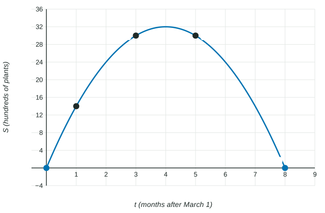
The same model comes from transformations. Its maximum is at $(4, 32)$ , so $S(t) = a(t - 4)^2 + 32$ ; the point $(0, 0)$ gives $0 = 16a + 32$ and $a = -2$ .

Regression: store every constant

Real data rarely fall exactly on a curve. A calculator regression (linear, quadratic, cubic or quartic in this unit) chooses the constants that bring the model closest to all the data at once. Enter the inputs and outputs as two lists, choose the regression type you justified from the data and context, and store the result.

Store, do not round. If $a = -2.589285...$ , keep every digit in the calculator and use the stored model for every later step. Give only the final answer correct to three decimal places. Rounding a constant early and then predicting with it is the most common way to lose a point on Question 2.

Using the model: values, rates and units

A prediction is an output with its unit: $S(6) = -72 + 96 = 24$ hundred plants. An average rate of change is output units per input unit.

Worked example 2. Find the average rate of change of $S$ on $[1, 3]$ and say what it means.

The average rate of change of $S$ on $[1, 3]$ is $\frac{S(3) - S(1)}{3 - 1}$ $= \frac{30 - 14}{2}$ $= 8$ hundred plants per month. It is the slope of the secant line through $(1, 14)$ and $(3, 30)$ .

In context: from month $1$ to month $3$ , sales rose by $8$ hundred plants per month on average.

Inverse proportion and inverse-square laws

Some contexts call for a rational model. If $y$ is inversely proportional to $x$ , then $y = \frac{k}{x}$ : doubling $x$ halves $y$ , as when more painters share a job. An inverse-square law, $y = \frac{k}{x^2}$ , divides $y$ by $4$ when $x$ doubles, as for the brightness of a light and your distance from it.

Worked example 3. Intensity $I$ is inversely proportional to the square of the distance $d$ , and $I = 200$ at $d = 3$ . Find $I(d)$ and $I(6)$ .

$I = \frac{k}{d^2}$ , so $200 = \frac{k}{9}$ and $k = 1800$ . Then $I(d) = \frac{1800}{d^2}$ and $I(6) = \frac{1800}{36} = 50$ .

The domain the context allows

A model is only trusted for inputs the situation allows. For $S(t) = -2t(t - 8)$ , the outputs are negative after $t = 8$ , and sales cannot be negative, so the model can be used for $0 \le t \le 8$ (see the figure). Name the bound and the reason, with the values. Also say why predictions far past the last data point are risky: the data no longer support the model there, and its shape (here, falling toward negative values) may not match what really happens.