Least-Squares Regression — AP® Statistics Notes

You can predict with a regression line and check it with residuals. Two questions remain. Which line, out of all the lines you could draw, should be used? And once you have it, how well does it do? This topic answers both, and then looks at the points that can change the answers.

The least-squares line

Every line through a scatterplot leaves residuals, some positive and some negative. Adding them up is useless, because they cancel. Squaring them first makes every miss count, and big misses count a lot. The least-squares regression line is the line that makes

$\sum (y - \hat{y})^2 = \sum \text{residual}^2$

as small as possible. Exactly one line does that, and technology finds it. Its slope and intercept have simple formulas in terms of summary statistics:

$b = r\frac{s_y}{s_x}, \qquad a = \bar{y} - b\bar{x}.$

Two facts follow. The line always passes through the point of means, $(\bar{x}, \bar{y})$ . And in standard deviation units, an $x$ that is one SD above $\bar{x}$ gets a prediction only $r$ SDs above $\bar{y}$ : predictions are pulled toward the mean unless $r = \pm 1$ . (The reference sheet gives $\hat{y} = a + bx$ but not the slope formula, so learn $b = r\frac{s_y}{s_x}$ as a relationship.)

Worked example 1. For ten basketball players, practice hours have $\bar{x} = 5.00$ , $s_x = 2.00$ ; free throw percentages have $\bar{y} = 61.40$ , $s_y = 6.04$ ; and $r = 0.966$ . Find the least-squares line.

Slope: $b$ $= 0.966\left(\frac{6.04}{2.00}\right)$ $= 2.917$ .

Intercept: $a$ $= 61.40 - 2.917(5.00)$ $= 46.82$ .

Line: $\hat{y} = 46.82 + 2.917x$ . For each additional hour of practice a week, the predicted free throw percentage increases by about 2.9 percentage points.

How well does the line fit? $r^2$ and $s$

The coefficient of determination, $r^2$ , compares the scatter around the line with the scatter around $\bar{y}$ . It is the fraction of the variation in $y$ that the line accounts for. Interpret it with this template:

"About [ $r^2$ as a percent] of the variation in [ $y$ ] is accounted for by the linear model using [ $x$ ]."

The standard deviation of the residuals, $s$ , is the typical size of a prediction error, in the units of $y$ :

"The actual [ $y$ ] typically differs from the predicted [ $y$ ] by about $s$ [units]."

Worked example 2. A magazine regresses fuel economy (mpg) on weight (thousands of pounds) for 30 car models. The output shows Constant 48.7, Weight $-6.25$ , S = 2.81 and R-Sq = 76.4%.

Line: $\widehat{\text{mpg}}$ $= 48.7 - 6.25(\text{weight})$ .

Slope: for each additional 1,000 pounds, the predicted fuel economy decreases by about 6.25 mpg.

$r^2$ : about 76.4% of the variation in fuel economy is accounted for by the linear model using weight.

$s$ : a car's actual fuel economy typically differs from its predicted fuel economy by about 2.81 mpg.

$r$ : $r = -\sqrt{0.764} = -0.874$ , negative because the slope is negative.

Reading output: the "Constant" row is the intercept $a$ , the row named for the explanatory variable is the slope $b$ , "S" is $s$ and "R-Sq" is $r^2$ . Output may show other columns; this course needs only these.

Unusual points

Practice hours against free throw percentage for ten players rising steeply, with slope 2.92 for their least-squares line; an eleventh player at 16 hours and 58% pulls the line down to a slope of 0.49. — **Figure 1.** One player far to the right pulls the least-squares line down. LevlPrep original diagram.

Kind of point	What it is	Typical effect
Outlier	a large residual: far above or below the line	raises $s$ , lowers $r$ and $r^2$
High-leverage point	an $x$ value far from $\bar{x}$	can pull the line toward itself
Influential point	removing it changes the slope or intercept a lot	often a high-leverage point

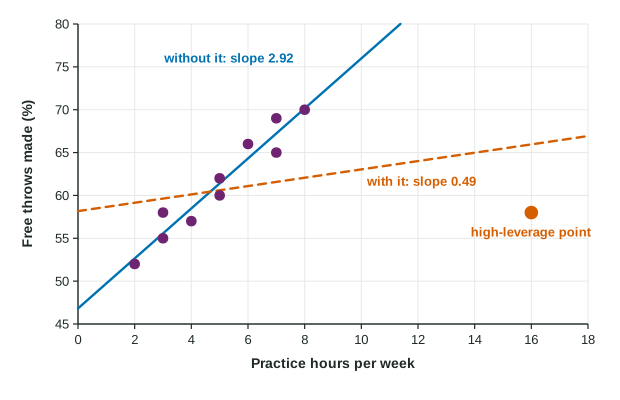
Because squares make far-off points count heavily, the least-squares line, like the mean, is not resistant. The figure shows the ten players plus an eleventh who practices 16 hours a week and makes 58%. With all eleven, the slope is 0.49 and $r = 0.32$ . Without the eleventh, the slope is 2.92 and $r = 0.97$ . That single high-leverage point is influential: it hides a strong linear association among everyone else.

A point near $\bar{x}$ with an unusual $y$ behaves differently. It has a large residual, so it raises $s$ and lowers $r$ , but it has little leverage, so the slope barely moves.

What to do with unusual points: look for a reason, then report the analysis with and without them. Never delete a point just because it does not fit.

The least-squares line

How well does the line fit? r2r^2 and ss

Unusual points

How well does the line fit? $r^2$ and $s$