Least-Squares Regression
The least-squares regression line makes the sum of squared residuals as small as possible; its slope is b = r(s_y)/(s_x) and it passes through (x-bar, y-bar) .
Part 1 · Hook
Why this matters
Part 2 · Before you start
What this builds on
Part 3 · Prerequisite check
Quick check before you start
1. A point is at and the line predicts 46 there. What is the residual?
Show the answer
.
- Correct: :
- :
- :
- :
2. A correlation of describes
- a strong negative linear association
- a weak negative association
- a strong positive association
- no association
Show the answer
Size near 1, negative sign.
- Correct: a strong negative linear association:
- a weak negative association:
- a strong positive association:
- no association:
Part 4 · See it
See it first
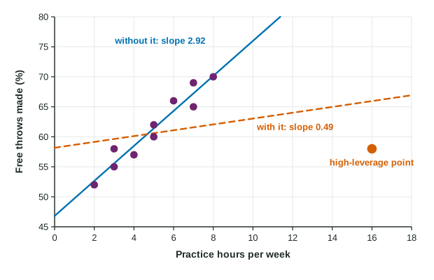
Part 5 · Step by step
How it works, step by step
- Every line leaves residuals; square them so misses above and below both countthe least-squares line is the one line that makes as small as possible
- Solving for that linegives and a line through , so
- Compare the scatter around the line with the scatter around is the share of the variation in the line accounts for, and is the typical size of a residual
- Squaring makes far-off points count heavilya point with an extreme value (high leverage) can pull the line toward itself and be influential
Part 6 · Key ideas
Key ideas
- The least-squares regression line minimizes the sum of squared residuals; and it passes through .
- : "About [ ]% of the variation in [y] is accounted for by the linear model using [x]."
- : "The actual [y] typically differs from the predicted [y] by about [units of y]."
- Outlier: a large residual. High-leverage point: an extreme . Influential point: removing it changes the slope or intercept a lot.
Part 7 · Misconception
A common mistake
Part 8 · Check yourself
Check yourself
Exam-style questions. Anything you miss goes into your review queue.
Table
Computer output: car weight and fuel economy
| Predictor | Coef |
|---|---|
| Constant | 48.7 |
| Weight | |
| S = 2.81 | R-Sq = 76.4% |
1. Which is the correct interpretation of the slope?
- For each extra 1,000 lb, predicted fuel economy drops by about 6.25 mpg
- For each additional 1,000 pounds, each car loses exactly 6.25 mpg
- A car that weighs 0 pounds is predicted to get 6.25 mpg
- For each additional pound of weight, the predicted fuel economy decreases by about 6.25 mpg
Show the answer
Slope in context with "predicted" and the units of .
- Correct: For each extra 1,000 lb, predicted fuel economy drops by about 6.25 mpg: Right: the slope is the predicted change in per one-unit increase in , and the unit of here is 1,000 pounds.
- For each additional 1,000 pounds, each car loses exactly 6.25 mpg: The slope describes predicted values, not an exact change for each car.
- A car that weighs 0 pounds is predicted to get 6.25 mpg: That mixes up the slope and the intercept, and a weight of 0 is not sensible.
- For each additional pound of weight, the predicted fuel economy decreases by about 6.25 mpg: Weight is in thousands of pounds, so one unit of is 1,000 pounds.
2. Which is the correct interpretation of R-Sq = 76.4%?
- About 76.4% of the variation in fuel economy is accounted for by the linear model using weight
- Weight causes about 76.4% of the variation in a car's fuel economy
- About 76.4% of the cars in the sample have fuel economy the line predicts correctly
- The correlation between weight and fuel economy for these 30 car models is 0.764
Show the answer
: "About [r squared]% of the variation in [y] is accounted for by the linear model using [x]."
- Correct: About 76.4% of the variation in fuel economy is accounted for by the linear model using weight: Right: is the fraction of the variation in explained by the line.
- Weight causes about 76.4% of the variation in a car's fuel economy: measures how much variation the line accounts for, not cause.
- About 76.4% of the cars in the sample have fuel economy the line predicts correctly: is not a share of cars; predictions are rarely exactly right.
- The correlation between weight and fuel economy for these 30 car models is 0.764: The correlation is , negative because the slope is negative.
3. Which is the correct interpretation of S = 2.81?
- A car's actual mpg is typically about 2.81 mpg away from its predicted mpg
- The predicted fuel economy changes by about 2.81 mpg for each additional 1,000 pounds
- About 2.81% of the variation in fuel economy is left unexplained
- The cars' weights typically differ from their mean weight by about 2.81 thousand pounds
Show the answer
: "The actual [y] typically differs from the predicted [y] by about [units]."
- Correct: A car's actual mpg is typically about 2.81 mpg away from its predicted mpg: Right: , the standard deviation of the residuals, is the typical size of a prediction error, in the units of .
- The predicted fuel economy changes by about 2.81 mpg for each additional 1,000 pounds: That would be a slope; the slope here is .
- About 2.81% of the variation in fuel economy is left unexplained: The unexplained share is ; is in mpg, not a percent.
- The cars' weights typically differ from their mean weight by about 2.81 thousand pounds: measures scatter around the line in units, not the spread of .
Table
Summary statistics for ten players
| Mean | Standard deviation | |
|---|---|---|
| Practice hours, | 5.00 | 2.00 |
| Free throws (%), | 61.40 | 6.04 |
| Correlation |
4. Write the expression for the slope of the least-squares line, , with the values substituted, then evaluate it.
Type the expression as on the exam, with the values substituted.
Show the answer
- Answer:
5. A player practices exactly 5 hours a week, the mean. What free throw percentage does the least-squares line predict?
- About 64.3%, one SD of above the mean of
- 46.8%, the intercept
- 5%, the mean of
- 61.4%, the mean of
Show the answer
at is .
- About 64.3%, one SD of above the mean of : At the prediction is exactly .
- 46.8%, the intercept: The intercept is the prediction at 0 hours, not at 5.
- 5%, the mean of : The prediction is in percent made, the variable.
- Correct: 61.4%, the mean of : Right: the least-squares line always passes through .
6. What makes the least-squares regression line "least squares"?
- It minimizes the sum of the squared residuals
- It passes through as many data points as possible
- It makes each residual as small as possible
- It has the smallest possible slope
Show the answer
Least squares: minimize .
- Correct: It minimizes the sum of the squared residuals: Right: among all lines, it gives the smallest .
- It passes through as many data points as possible: It may pass through none of the points.
- It makes each residual as small as possible: No line can make every residual small; it minimizes the sum of their squares.
- It has the smallest possible slope: The slope is whatever minimizes the squared residuals.
Part 9 · Summary
Summary
Part 10 · Up next
What comes next
This is the last topic in the course.
Part 11 · Connections