Reasoning with Slope Fields — AP® Calculus AB Notes

Once a slope field is drawn, you can read it like a weather map. It shows where solutions rise and fall, where they level off, and where they head in the long run, all without a formula. This page shows how to sketch the solution curve through a point, how to spot equilibrium solutions, and how to find the concavity of a solution from the differential equation itself.

Sketching the solution through a point

Put your pencil on the given point. The segment there shows which way to go. Move a little, look at the nearby segments, adjust, and keep going. Then go back to the point and do the same in the other direction. Rules that keep the sketch honest:

Pass exactly through the given point. The point $(0, 5)$ has $x = 0$ and $y = 5$ ; do not start at $(5, 0)$ .
Follow the segments: the curve should be tangent to the segments it passes, never cutting across them.
Extend the curve across the whole field shown, to the left and to the right of the point.
Do not cross a row of horizontal segments that forms an equilibrium solution (next section).

The slope field of dy/dx = (3 − y)/2 drawn every half unit. The dashed green line y = 3 has slope 0 everywhere. A crimson curve through (0, 1) rises and flattens toward y = 3; a blue curve through (0, 5.5) falls and flattens toward y = 3. Neither crosses the line. — **Figure 1.** The slope field of $\frac{dy}{dx} = \frac{3 - y}{2}$ with the solutions through $(0, 1)$ and $(0, 5.5)$ . Both approach the line $y = 3$ without crossing it. LevlPrep original diagram.

Equilibrium solutions

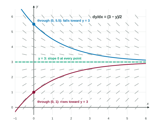
Sometimes a whole horizontal line is made of flat segments. For $\frac{dy}{dx} = \frac{3 - y}{2}$ , every point with $y = 3$ has slope 0. Then the constant function $y = 3$ is itself a solution: its derivative is 0, and the right side is 0 too. A constant solution like this is an equilibrium solution.

To find them, set the right side equal to 0 and solve for $y$ . The answer must work for every $x$ . For $\frac{dy}{dx} = x^2(y - 3)(y + 1)$ the equilibrium solutions are $y = 3$ and $y = -1$ . The factor $x^2$ also makes the slope 0 along $x = 0$ , but a vertical line is not a function of $x$ , so it is not a solution.

Equilibrium solutions organize everything else. When the right side of the equation is a smooth formula in $x$ and $y$ , as in every slope field on this page, two solution curves never cross or touch. (A right side with $\sqrt{y}$ , such as a draining tank's $\frac{dh}{dt} = -\frac{1}{5}\sqrt{h}$ , is the exception at $h = 0$ : the tank empties and the depth stays at 0.) So a solution that starts below $y = 3$ stays below it. In the figure, slopes below 3 are positive and get gentler near 3, so the curve through $(0, 1)$ rises and flattens toward 3. Above 3 the slopes are negative, so the curve through $(0, 5.5)$ falls toward 3. Both approach 3 as $x$ grows.

Not every equilibrium attracts. For $\frac{dy}{dx} = \frac{y - 1}{2}$ , slopes are positive above $y = 1$ and negative below it, so solutions move away from $y = 1$ on both sides. A solution through $(0, 2)$ rises faster and faster; one through $(0, 0)$ falls without bound.

Increasing, decreasing and extrema

The sign of $\frac{dy}{dx}$ says where a solution rises or falls, exactly as for any function. For $\frac{dy}{dx} = x(2 - y)$ and points below $y = 2$ , the factor $2 - y$ is positive, so the slope has the sign of $x$ : negative left of the $y$ -axis, positive right of it. A solution crossing the $y$ -axis below $y = 2$ therefore has a relative minimum there, because $\frac{dy}{dx}$ changes from negative to positive.

Concavity: the second derivative by the chain rule

To decide whether a solution curve is concave up or down, you need $\frac{d^2y}{dx^2}$ . Differentiate the right side of the equation with respect to $x$ , remembering that $y$ is a function of $x$ . So every $y$ you differentiate brings a factor $\frac{dy}{dx}$ , and then you replace $\frac{dy}{dx}$ by the right side of the equation.

Worked example. A solution of $\frac{dy}{dx} = y^2 - x$ passes through $(1, 2)$ . Is it concave up or down there?

Differentiate both sides with respect to $x$ : $\frac{d^2y}{dx^2} = 2y\frac{dy}{dx} - 1$ . The $2y\frac{dy}{dx}$ comes from the chain rule on $y^2$ .

At $(1, 2)$ : $\frac{dy}{dx} = 2^2 - 1 = 3$ . So $\frac{d^2y}{dx^2}$ $= 2(2)(3) - 1$ $= 11$ .

Since $\frac{d^2y}{dx^2} = 11 > 0$ , the solution curve is concave up at $(1, 2)$ .

The classic slip is to write $\frac{d}{dx}(y^2) = 2y$ , or even 0 "because there is no $x$ ". Both forget that $y$ changes as $x$ changes. For $\frac{dy}{dx} = \frac{y - 1}{2}$ the correct second derivative is $\frac{1}{2}\frac{dy}{dx} = \frac{y - 1}{4}$ , not 0.

Worked example 2. For $\frac{dy}{dx} = x(2 - y)$ , find $\frac{d^2y}{dx^2}$ in terms of $x$ and $y$ .

Product rule: $\frac{d^2y}{dx^2}$ $= 1 \cdot (2 - y) + x \cdot \left(-\frac{dy}{dx}\right)$ .

Substitute $\frac{dy}{dx} = x(2 - y)$ : $\frac{d^2y}{dx^2}$ $= (2 - y) - x^2(2 - y)$ $= (2 - y)(1 - x^2)$ .

Long-run behavior

In context, an equilibrium solution is often a value the quantity settles at. A drink with $\frac{dT}{dt} = -0.1(T - 65)$ warms or cools toward 65 °F, the room temperature. Read the long run from the signs: below the equilibrium the rate is positive, above it negative, so the temperature approaches 65 from either side.