Functions and Their Graphs — AP® Calculus AB Notes

Calculus is the study of how functions change and how they add up. Every exam question hands you a function in some form: a formula, a graph, a table of values or a sentence about a real situation. If you are a little rusty from precalculus, this page is for you. It covers exactly the function skills the course uses, with the habits that save points later.

A function is a rule with one output per input

A function takes an input and gives back exactly one output. We write $f(x)$ for the output when the input is $x$ . The letter $x$ is just a placeholder: $f(x) = x^2 - 3x$ means "square the input, then subtract three times the input."

To evaluate, replace every $x$ with the input, in parentheses. The parentheses matter most when the input is negative or is itself an expression. That habit, kept all year, prevents a whole family of sign mistakes.

Worked example 1. Let $f(x) = x^2 - 3x$ . Find $f(-2)$ and $f(a + 1)$ .

$f(-2)$ $= (-2)^2 - 3(-2)$ $= 4 + 6$ $= 10$ . Without parentheses, $-2^2$ would read as $-4$ , which is wrong.

$f(a + 1)$ $= (a + 1)^2 - 3(a + 1)$ $= a^2$ $+ 2a$ $+ 1 - 3a - 3$ $= a^2 - a - 2$ .

Notice that $f(a + 1)$ is not $f(a) + 1$ . A function acts on the whole input at once.

Domain and range

The domain is the set of inputs the rule accepts. The range is the set of outputs it actually produces. For the functions in this course, two things shrink a domain:

A denominator can never be 0.
A square root (or any even root) needs a number that is 0 or more.

Worked example 2. Find the domain of $h(x)$ $= \frac{\sqrt{x + 4}}{x - 1}$ .

The root needs $x + 4 \ge 0$ , so $x \ge -4$ . The denominator needs $x - 1 \ne 0$ , so $x \ne 1$ .

Domain: $x \ge -4$ and $x \ne 1$ . Notice that $x = -4$ is allowed: $\sqrt{0} = 0$ is fine on top.

Reading a graph

The graph of $f$ is every point $(x, f(x))$ . So $f(a)$ is a height: go to $x = a$ on the horizontal axis and read how high the graph is there.

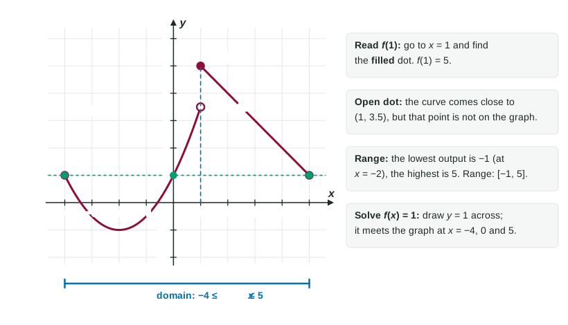
Graph of a piecewise function f from x = -4 to x = 5: a parabola piece from the filled point (-4, 1) down to (-2, -1) and up toward an open circle at (1, 3.5), then a line from the filled point (1, 5) down to the filled point (5, 1). Notes beside it: f(1) = 5 is the filled dot; the open circle is not on the graph; the range is from -1 to 5; the line y = 2 meets the graph at x = 0 and x = 4. — **Figure 1.** One graph, four readings: a value, an open circle, the range, and the solutions of an equation. LevlPrep original diagram.

Graphs in calculus often have pieces, so learn the two kinds of dot. A filled dot is a point on the graph. An open circle marks a point the graph comes close to but does not include. In the figure, the open circle at $(1, 3.5)$ is not on the graph; the filled dot at $(1, 5)$ is, so $f(1) = 5$ .

Three more readings you will use constantly:

Solve $f(x) = k$ : draw the horizontal line $y = k$ and read the $x$ -values where it meets the graph.
Where is $f$ positive? Where the graph is above the $x$ -axis.
Range: the lowest and highest heights, minding open circles at the ends.

Piecewise functions

A piecewise function uses different formulas on different parts of its domain: $f(x) = \begin{cases} x^2 & x < 2 \\ 3x - 1 & x \ge 2 \end{cases}$ To evaluate, first decide which piece the input belongs to, then use only that formula. The boundary value goes wherever the "or equal to" sign is. Here $f(2)$ uses $3x - 1$ , so $f(2) = 5$ , while $f(1.9) = 3.61$ uses $x^2$ . Calculus cares a lot about what happens at boundaries like $x = 2$ , so slow down there.

Lines and slope

The slope of a line is rise over run. Through $(x_1, y_1)$ and $(x_2, y_2)$ : $m = \frac{y_2 - y_1}{x_2 - x_1}$ Subtract in the same order on top and bottom. A positive slope means the line goes up to the right; a negative slope, down.

Calculus writes lines in point-slope form, because it usually knows one point and the slope there: $y - y_1 = m(x - x_1)$ You do not need to rearrange it into $y = mx + b$ unless a question asks; the exam accepts point-slope form.

Worked example 3. Find the line through $(1, 4)$ and $(3, -2)$ .

Slope: $m$ $= \frac{-2 - 4}{3 - 1}$ $= \frac{-6}{2}$ $= -3$ .

Point-slope form with $(1, 4)$ : $y - 4 = -3(x - 1)$ . If you want it: $y = -3x + 7$ .

Check with the other point: $-3(3) + 7 = -2$ . Correct.

Composite functions

A composite function feeds the output of one function into another. $f(g(x))$ means: apply $g$ first, then apply $f$ to the result. Work from the inside out.

Worked example 4. Let $f(x) = x^2$ and $g(x) = 3x - 1$ . Find $f(g(x))$ and $g(f(x))$ .

$f(g(x))$ $= f(3x - 1)$ $= (3x - 1)^2$ . Square the whole input.

$g(f(x))$ $= g(x^2)$ $= 3x^2 - 1$ . Different! The order of composition matters.

Going backward is just as useful. $h(x) = \sqrt{x^2 + 1}$ is $f(g(x))$ with inside $g(x) = x^2 + 1$ and outside $f(x) = \sqrt{x}$ . In Unit 3 you will split functions this way all the time.

Moving graphs

A graph transformation changes a known graph in a predictable way:

Formula	What happens to the graph of $f$
$f(x) + k$	moves up $k$ (down if $k < 0$ ): a vertical shift
$f(x - h)$	moves right $h$ (left if $h < 0$ ): a horizontal shift
$-f(x)$	flips over the $x$ -axis
$a f(x)$	stretches vertically by the factor $a$

The parabola y = x squared, dashed, with lowest point (0, 0), and the parabola y = (x - 2) squared + 1, solid, with lowest point (2, 1): the same shape moved 2 right and 1 up. — **Figure 2.** $y = (x - 2)^2 + 1$ is $y = x^2$ moved right 2 and up 1. LevlPrep original diagram.

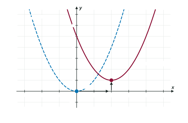
The horizontal shift feels backward: $x - 2$ moves the graph right. Here is why. The new graph reaches the old graph's lowest point when $x - 2 = 0$ , that is, at $x = 2$ .

Polynomials, rational functions and asymptotes

A polynomial is a sum of terms like $5x^3$ or $-2x$ , with whole-number powers. Its domain is every real number. A rational function is one polynomial divided by another, such as $r(x) = \frac{2x + 1}{x - 4}$ . Its domain leaves out every zero of the denominator.

An asymptote is a line the graph approaches. For a rational function:

Where the denominator is 0 and the numerator is not, there is a vertical asymptote. For $r$ , that is $x = 4$ (the numerator is 9 there).
When top and bottom have the same degree, the outputs settle near the ratio of the leading coefficients as $|x|$ grows large: a horizontal asymptote. For $r$ , that is $y = \frac{2}{1} = 2$ . When the top has lower degree, the horizontal asymptote is $y = 0$ .

When the top and bottom are both 0 at the same $x$ , something more interesting happens. Unit 1 is largely about that case.