To detect evolution, you need to know what "not evolving" looks like. The Hardy-Weinberg principle supplies exactly that: the allele and genotype frequencies of a population in which nothing is changing them. This page derives the two equations, shows how to use them, lists the five conditions, and explains how departures from the expected frequencies reveal which forces are at work.
The question: why don't dominant alleles take over?
In 1908 Reginald Punnett, of the Punnett square, was asked why short fingers, caused by a dominant allele, had not spread through the human population. He passed the question to the mathematician G. H. Hardy. Hardy showed, as did the physician Wilhelm Weinberg independently that same year, that dominance has nothing to do with how common an allele becomes. In a large population mating at random, allele frequencies stay the same in every generation unless something changes them. That steady state is Hardy-Weinberg equilibrium.
The two equations
Take one gene with two alleles, A and a. Let p be the frequency of A and q the frequency of a. Every copy of the gene is one or the other, so:
p + q = 1
If the population mates at random, each new individual is formed by two gametes drawn at random from the population's gamete pool, where a fraction p carry A and q carry a. By the product rule, the chance of drawing A then A is p × p = p², and a then a is q². A heterozygote can form two ways (A from the egg and a from the sperm, or the reverse), so its chance is pq + qp = 2pq. The three genotypes cover every possibility, so:
p² + 2pq + q² = 1 (AA + Aa + aa)
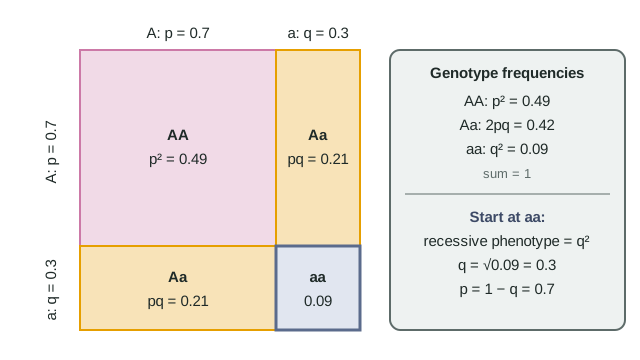
Figure 1 draws this as a Punnett square for a whole population. Now follow one more generation. AA individuals make only A gametes, aa only a, and Aa make half of each. The share of A gametes is p² + ½(2pq) = p² + pq = p(p + q) = p. The allele frequency is unchanged, and so are the genotype frequencies after the next round of random mating. Dominance appears nowhere in the arithmetic.
Worked example 1: from genotype counts. A sample of 500 plants has 245 AA, 210 Aa and 45 aa. Is it consistent with equilibrium?
Step 1, allele frequencies. Copies of A = (2 × 245) + 210 = 700 of 1,000, so p = 0.70 and q = 0.30.
Step 2, expected genotype frequencies. p² = 0.49, 2pq = 2 × 0.70 × 0.30 = 0.42, q² = 0.09.
Step 3, expected counts. 0.49 × 500 = 245 AA, 0.42 × 500 = 210 Aa, 0.09 × 500 = 45 aa. Observed and expected match exactly, so this sample shows no departure from equilibrium.
Worked example 2: from a recessive phenotype. In a population assumed to be at equilibrium, 16% of the moths have white wings, a recessive trait. How many of 1,000 moths are expected to be heterozygous?
Step 1. White moths are aa, so q² = 0.16. Step 2. q = √0.16 = 0.40, and p = 1 − 0.40 = 0.60. Step 3. 2pq = 2 × 0.60 × 0.40 = 0.48, so about 480 of 1,000 moths are expected to be Aa. Notice the order: start from q², the one genotype you can see. You cannot start from the dominant phenotype, because it lumps AA and Aa together.
More practice with new numbers, including testing observed counts with chi-square, is in the next skills lesson, Hardy-Weinberg calculations, and the Hardy-Weinberg calculations practice tool.
The five conditions
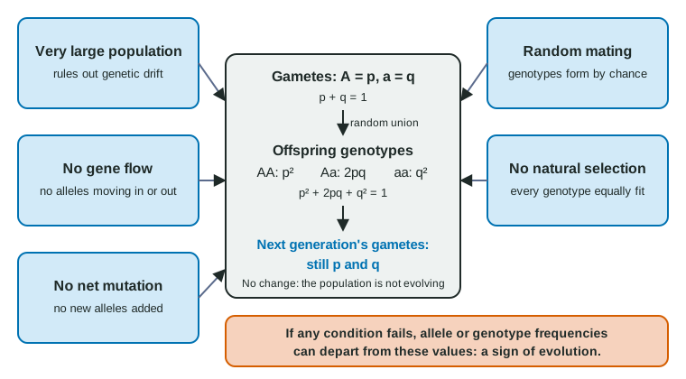
The argument above assumed that nothing except random mating shapes the next generation. Spelled out, that means five Hardy-Weinberg conditions (Figure 2), each ruling out one process from topic 7.4:
| Condition | Process it rules out | What failure does |
|---|---|---|
| Very large population | Genetic drift | Allele frequencies wander at random; alleles can be lost or fixed |
| No gene flow | Migration of alleles in or out | Allele frequencies move toward those of the source population |
| No net mutation | Mutation adding or changing alleles | Very slow change in allele frequencies |
| Random mating | Nonrandom mating (inbreeding, assortative mating) | Too many homozygotes and too few heterozygotes, though allele frequencies stay the same |
| No natural selection | Differences in survival or reproduction among genotypes | Allele frequencies shift toward the fitter alleles; genotype counts among survivors can depart from p², 2pq, q² |
No real population meets all five perfectly. That is not a flaw: the equations are a null hypothesis. They say what you would see if nothing were happening, so a departure tells you something is.
Reading a departure
A deviation from Hardy-Weinberg is a difference between observed and expected frequencies too large to blame on chance in sampling, which is usually judged with a chi-square test. The shape of the difference is a clue to the cause:
- Too few heterozygotes, both homozygotes in excess. Typical of inbreeding or self-fertilization, which pair like alleles. (Sampling two separate populations as if they were one does the same.)
- Too many heterozygotes. Suggests selection that favors heterozygotes, for example when both homozygotes survive less well. In parts of Africa, adults carrying one sickle-cell allele survive malaria better than people with two normal alleles, and people with two sickle-cell alleles often die young, so adult samples there contain more heterozygotes than q predicts. Newborns, before selection has acted, fit the equations.
- Allele frequencies changing over generations. Selection, drift, gene flow or, very slowly, mutation. Which one takes other evidence: replicate populations moving randomly point to drift, a steady trend linked to the environment to selection, movement toward a neighbor's frequencies to gene flow.
Two more things follow from the equations. First, a population can fit the equations at one moment and still be evolving across generations; you need data from more than one generation to see a trend. Second, selection against a rare recessive allele is slow. When q is small, almost every copy of the allele sits in a heterozygote, where it is not exposed to selection. At q = 0.10, the fraction of a alleles carried by heterozygotes is 2pq ÷ (2pq + 2q²) = p = 0.90: nine copies in ten are hidden. That is why harmful recessive alleles persist for many generations. Watch this, and the effect of population size, in the Hardy-Weinberg and genetic drift simulator.