A rate law (topic 5.2) tells you the rate at one moment. Often you want something else: how much reactant is left after 10 minutes, or how long until half of it is gone. The integrated rate laws answer those questions. They also give the cleanest way to find the order from a single experiment: make the right graph and see which one is a straight line. This topic uses natural logarithms; the "Logarithms" page just before it covers ln and e.
Three orders, three equations
| Order | Rate law | Integrated rate law | Straight-line plot | Slope |
|---|---|---|---|---|
| 0 | rate = k | [A]t = [A]0 − kt | [A] vs t | −k |
| 1 | rate = k[A] | ln[A]t − ln[A]0 = −kt | ln[A] vs t | −k |
| 2 | rate = k[A]² | 1/[A]t − 1/[A]0 = kt | 1/[A] vs t | +k |
[A]0 is the starting concentration and [A]t the concentration at time t. The first-order law can also be written [A]t = [A]0e−kt. The exam's equations sheet gives the first- and second-order laws and the first-order half-life. It does not give the zero-order law, so learn it: it just says the concentration falls by the same amount every second.
Finding the order from a graph
Each integrated law has the shape y = mx + b, so one of three graphs comes out straight (Figure 1):
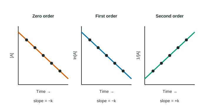
Plot [A], ln[A] and 1/[A] against time. Whichever plot is linear tells you the order, and its slope gives k. When you justify an order, name the plot: "The plot of ln[A] against time is linear, so the reaction is first order." "The graph is linear" earns nothing on its own, because every order has a linear graph of something.
From a table, you can check without drawing: if ln[A] changes by the same amount in each equal time step, ln[A] vs t is linear. If 1/[A] changes by the same amount each step, 1/[A] vs t is linear.
Worked example: order and k from data
A compound decomposes at constant temperature. [A] = 0.800 M at 0 min, 0.400 M at 20 min, 0.200 M at 40 min.
Step 1: test each plot. [A] drops 0.400, then 0.200: not equal, so [A] vs t is not linear. 1/[A] = 1.25, 2.50, 5.00 M⁻¹: steps of 1.25, then 2.50, not equal. ln[A] = −0.223, −0.916, −1.609: steps of −0.693 each time. ln[A] vs t is linear, so the reaction is first order.
Step 2: k from the slope. slope = (−1.609 − (−0.223))/(40 min − 0 min) = −1.386/40 min = −0.0347 min⁻¹. k = −slope = 0.0347 min⁻¹.
Step 3: predict. At 60 min: ln[A] = ln(0.800) − (0.0347 min⁻¹)(60 min) = −0.223 − 2.08 = −2.30, so [A] = e−2.30 = 0.100 M.
Half-life
The half-life, t½, is the time for a reactant's concentration to fall to half its value. Put [A]t = ½[A]0 into the first-order law: ln(½) = −kt½, and ln 2 = 0.693, so
t½ = 0.693 / k (first order)
The starting concentration is not in this equation. A first-order reaction takes the same time to go from 1.00 M to 0.50 M as from 0.50 M to 0.25 M. In the worked example, the concentration halves every 20 min: 0.693/0.0347 min⁻¹ = 20.0 min.
Radioactive decay is first order. After n half-lives, (½)n of the sample is left: after 3 half-lives, 12.5%.
For a second-order reaction the half-life is not constant: it gets longer as the reaction goes on, because the rate falls with [A]². For zero order it gets shorter. You only need the first-order formula; for the others, reason from the integrated law.
Worked example: second order
2 HI(g) → H₂(g) + I₂(g) is second order in HI with k = 0.0300 M⁻¹ s⁻¹. Starting from [HI] = 0.500 M, find [HI] after 100. s.
1/[HI]t = kt + 1/[HI]0 = (0.0300 M⁻¹ s⁻¹)(100. s) + 1/(0.500 M) = 3.00 M⁻¹ + 2.00 M⁻¹ = 5.00 M⁻¹.
[HI]t = 1/(5.00 M⁻¹) = 0.200 M.
Common slips
- Using log (base 10) in place of ln. The integrated rate laws use the natural log.
- Getting the sign of the slope wrong: −k for the [A] and ln[A] plots, +k for the 1/[A] plot. k itself is always positive.
- Writing "the graph is linear" without saying which graph.
- Using t½ = 0.693/k for a reaction that is not first order.