The Normal Curve and Percentiles — AP® Psychology Notes

Measure the heights of a thousand adults, or give a well-built test to a thousand students, and a picture appears: most values pile up near the middle and fewer and fewer appear toward the extremes. That shape is the normal curve. Intelligence test scores are built to follow it, and the exam asks you to read it.

The shape

A normal curve is a symmetric, bell-shaped frequency distribution. Because it is symmetric, the mean, the median and the mode all sit at the same point, the peak in the middle. Why does this shape show up so often? Many traits are the sum of many small, separate influences, and small influences pushing up and down tend to cancel, leaving most people near the middle.

The 68-95-99.7 rule

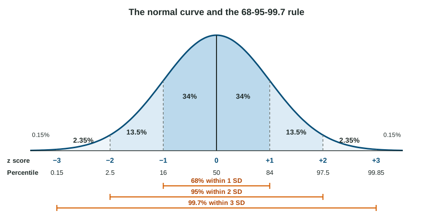
A bell-shaped normal curve with vertical lines at the mean and at 1, 2 and 3 standard deviations on each side. The bands hold 34% of scores between the mean and 1 SD on each side, 13.5% between 1 and 2 SD, 2.35% between 2 and 3 SD, and 0.15% beyond 3 SD. Below the axis, z scores run from minus 3 to plus 3, with percentiles 0.15, 2.5, 16, 50, 84, 97.5 and 99.85. Brackets show 68% of scores within 1 SD of the mean, 95% within 2 SD and 99.7% within 3 SD. — **Figure 1.** The normal curve, marked at each standard deviation. LevlPrep original diagram.

Mark the mean, then each standard deviation on both sides. In any normal distribution:

about 68% of scores lie within 1 standard deviation of the mean (34% on each side);
about 95% lie within 2 standard deviations (add 13.5% on each side);
about 99.7% lie within 3 standard deviations (add 2.35% on each side);
the last 0.15% on each side lies beyond 3 standard deviations.

So the bands from the middle out are 34, 13.5, 2.35 and 0.15. Every question about shares under the curve is solved by adding bands.

Worked example: shares under the curve. A reading test has a mean of 100 and a standard deviation of 15.

Between 85 and 115? That is 1 SD below to 1 SD above: $34 + 34 = 68\%$ .

Above 130? 130 is 2 SDs above. Above it: $2.35 + 0.15 = 2.5\%$ .

Below 85? Below the mean is 50%; take away the 34% between 85 and 100: $50 - 34 = 16\%$ .

The slip readers see most: giving one side when the question covers both (34% instead of 68%), or both sides when it covers one.

z scores

A z score says how many standard deviations a score is from the mean:

$z = \frac{x - \bar{x}}{\text{SD}}$

Above the mean, z is positive; below, negative; at the mean, zero. Because every test's scores are turned into the same units, z scores let you compare across tests.

Worked example: which score is better? Ana scored 72 in biology (mean 60, SD 6) and 85 in history (mean 80, SD 10).

Biology: $z$ $= \frac{72 - 60}{6}$ $= \frac{12}{6}$ $= 2$ .

History: $z$ $= \frac{85 - 80}{10}$ $= \frac{5}{10}$ $= 0.5$ .

The lower raw score, 72, is the better result: two standard deviations above the class, against half a standard deviation in history.

Percentile ranks

A percentile rank is the percent of scores below a given score. At the mean it is 50. One standard deviation above the mean is $50 + 34 = 84$ , the 84th percentile; one below is $50 - 34 = 16$ . Two above is $50 + 34 + 13.5 = 97.5$ .

A percentile is not the percent of questions right. A student who answered 70% of a very hard test correctly might be at the 95th percentile, because almost everyone else did worse.