
A study of 200 people produces 200 numbers. Nobody can read them one by one, so researchers summarize them: where the center is, and how spread out the values are. These are descriptive statistics. On the exam you work them out by hand, with no calculator, so the data sets are small.
The center: mean, median and mode
| How to find it | Best when | Watch out | |
|---|---|---|---|
| Mean, | add every value, divide by how many | the data are roughly symmetric, with no outliers | pulled toward outliers and toward the tail of a skewed distribution |
| Median | put the values in order, take the middle one | there are outliers or a skew | with an even count, average the two middle values |
| Mode | the most frequent value | categories, or the most common answer | there can be two modes (bimodal) or more |
Worked example: mean, median and mode by hand.
Six students recalled 4, 9, 6, 6, 12 and 5 words.
Mean. Add:
Median. Order the list first: 4, 5, 6, 6, 9, 12. Six values, so the middle falls between the 3rd and 4th: words.
Mode. 6 appears twice; every other value once. The mode is 6.
The two slips readers see most: giving the total (42) instead of the mean, and taking the middle of the list before putting it in order.
Outliers and skew
An outlier is a value far from the rest. Why does it matter so much for the mean? The mean uses the size of every value, so one huge value adds a lot to the total. The median only cares about which value is in the middle, so one huge value just becomes "the biggest" and the middle barely moves.
Worked example: one sneeze.
A participant's reaction times on 10 trials: 280, 280, 300, 300, 300, 300, 320, 320, 320 and 900 ms (the 900 was a sneeze).
Mean: the total is , so ms. That is slower than nine of the ten trials.
Median: the 5th and 6th values in order are both 300, so the median is 300 ms. It describes this person's usual speed much better.
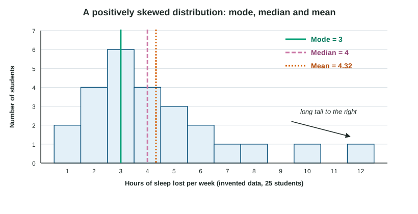
When a few extreme values stretch one side of a distribution, it is a skewed distribution, named for the direction of its tail. Income is positively skewed: most people earn moderate amounts and a few earn enormous amounts, so the tail stretches right and the mean is above the median. Scores on an easy test are negatively skewed: most are high, a few are low, and the mean falls below the median. Remember: the mean follows the tail.
A bimodal distribution has two peaks. It often means two groups are mixed together, such as students who did and did not read the book.
Spread: range and standard deviation
Two classes can both average 75 and still be very different: one where everybody scored 70 to 80, one where scores ran from 40 to 100. Measures of variation capture this.
The range is the highest value minus the lowest. It is quick, but it depends on just two values, so one outlier can stretch it.
The standard deviation (SD) is roughly the typical distance of the scores from the mean. A small SD means scores huddle near the mean; a large SD means they are spread out. On the exam you will read and compare standard deviations rather than compute them.
A frequency distribution lists how often each value or range of values occurs. A histogram draws it as touching bars, and its shape shows symmetry, skew or two peaks at a glance.