SRAS slopes up because wages and some prices are stuck for a while. But contracts end, wages are renegotiated, and suppliers reset their prices. Once everything has adjusted, does a higher price level still make the economy produce more? This page answers no, and shows what supply looks like in the long run.
When every price has adjusted
Suppose the price level rises by 10 percent. In the short run, firms earn more per unit while wages are fixed, so they produce more. Workers notice that their pay buys less and, when their contracts come up, they bargain for 10 percent more. Suppliers raise their prices too. Once costs have risen as much as selling prices, producing extra output is no more profitable than before, and firms go back to the output they produced at the start.
That output is full-employment output (potential output, YF): what the economy produces when unemployment is at its natural rate. In the long run, real output returns to YF whatever the price level. So long-run aggregate supply (LRAS) is a vertical line at YF.
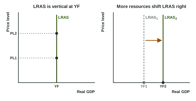
In the left graph, PL1 and PL2 both go with the same real output, YF. Use the same axes as before, Price level and Real GDP, and label the line LRAS with YF marked where it meets the horizontal axis.
Short run and long run side by side
| SRAS | LRAS | |
|---|---|---|
| Time frame | short run: nominal wages and some prices are sticky | long run: all wages and prices have adjusted |
| Shape | slopes up | vertical at YF |
| A higher price level | raises output (movement along SRAS) | leaves output at YF |
| Shifted by | input prices, productivity, taxes and rules on firms, wage bargaining | the quantity and quality of resources, and technology |
What shifts LRAS: the same things that shift the PPC
LRAS stands where the economy's resources, fully employed, put it. It moves only when that capacity changes (the right graph):
- Labor: more adults in the labor force, or workers with more education and skill.
- Capital: more factories, machines, roads and power plants.
- Land and natural resources: new reserves found, or farmland lost to drought for good.
- Technology: better ways to combine the same resources.
These are the same changes that shift the production possibilities curve outward in Unit 1. A point on the PPC means every resource is fully and efficiently used; that is full-employment output, so it is where LRAS stands. When LRAS shifts right, the PPC shifts out, and when a disaster destroys capital, LRAS shifts left and the PPC shifts in.
Worked example: did LRAS move? Country L's full-employment real GDP is 500 billion dollars in 2000, 550 in 2010 and 520 in 2020.
- 2000 to 2010: YF rose by billion, which is . LRAS shifted right.
- 2010 to 2020: the labor force stayed the same but the stock of machines fell, and YF fell to 520. LRAS shifted left.
- Check the cause, not the price level: in both cases the move came from resources, never from a change in the price level, which would only move the economy up or down the vertical line.
Common slip: shifting LRAS when spending changes ("consumers spend more, so LRAS shifts right"). More spending shifts AD. LRAS moves only with resources and technology. A second slip is drawing LRAS sloped: in the long run it is a vertical line at YF.
Some events move both supply curves at once. An earthquake that destroys factories raises costs right away (SRAS shifts left) and lowers what full employment can produce (LRAS shifts left). A lasting rise in productivity lowers costs and raises capacity, so both shift right. Ask two questions: does this change costs now (SRAS), and does it change what the economy can produce once everything adjusts (LRAS)?