You now have three curves: aggregate demand (what buyers plan to spend), short-run aggregate supply (what firms supply while wages are sticky) and long-run aggregate supply (what the economy produces at full employment). Put them on one graph and you have the AD-AS model, the graph behind most of the long free-response questions on the exam.
Drawing the AD-AS graph
- Vertical axis: Price level (PL). Horizontal axis: Real GDP (Y, or real output). Never "price" or "quantity", which belong to one market.
- AD slopes down, SRAS slopes up, LRAS is vertical at full-employment output, labeled YF on the horizontal axis.
- Mark the equilibrium the question asks for with dashed lines to both axes, labeled PL1 and Y1.
Short-run and long-run equilibrium
Short-run equilibrium is where AD crosses SRAS. At that price level, the real output buyers plan to purchase equals the real output firms are willing to supply. If the price level were higher, firms would supply more than buyers want and unsold goods would pile up; if lower, buyers would want more than firms supply. Either way the price level moves toward PL1.
That short-run point need not be at full employment. Long-run equilibrium is the special case where AD and SRAS cross on LRAS: real GDP equals full-employment output and unemployment equals the natural rate of unemployment.
Gaps: where Y1 stands against YF
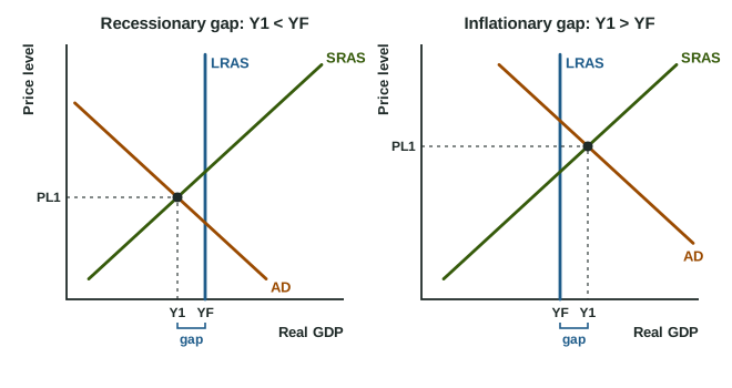
Compare short-run output Y1 with YF (the two graphs):
| Recessionary gap | Long-run equilibrium | Inflationary gap | |
|---|---|---|---|
| Output | Y1 < YF (left of LRAS) | Y1 = YF (on LRAS) | Y1 > YF (right of LRAS) |
| Unemployment | above the natural rate (cyclical unemployment) | equal to the natural rate | below the natural rate |
| Also called | a negative output gap | full employment | a positive output gap |
| What it feels like | idle factories, layoffs | normal times | overtime, labor shortages, prices pushed up |
Output above full employment is possible for a while: workers put in overtime, firms run machines extra shifts, and unemployment falls below its natural rate. It cannot last once wages catch up, which a later topic shows.
Worked example: read the gap. Alta's real GDP is 940 billion dollars, its full-employment real GDP is 1,000 billion dollars, and its unemployment rate is 7.5% against a natural rate of 5%.
- Compare outputs: 940 is less than 1,000, so Y1 is left of LRAS: a recessionary gap.
- Size in dollars: billion dollars.
- Size as a percent of full-employment output: .
- Check with unemployment: 7.5% is above the natural rate, so there are 2.5 points of cyclical unemployment, as a recessionary gap predicts.
Common slip: treating every AD-SRAS crossing as full employment ("the economy is in equilibrium, so there is no unemployment problem"). Equilibrium in the short run only means spending equals output supplied. Check where the crossing sits against LRAS, and remember that full employment still leaves natural unemployment.
Labels readers look for
A full-credit AD-AS graph has both axes labeled, all three curves labeled, LRAS drawn vertical at YF, and the short-run equilibrium marked as PL1 and Y1 with Y1 on the correct side of YF. If the question names a gap, draw Y1 where the gap puts it: left of YF for a recessionary gap, right of YF for an inflationary gap. Labeling the axes "P" and "Q" costs the graph point even when every curve is right.