A population is a group of individuals of one species living in the same area at the same time. Ecologists ask simple questions about it: how many are there, how are they spread out, and how fast is the number changing? This page shows how to measure a population, how births and deaths set its growth rate, why unchecked growth speeds up, and how a species' life history shapes all of this. The formulas are on the exam's formula sheet.
Measuring a population: density and dispersion
Population density is the number of individuals per unit area (or volume): 4 dandelions per square meter, 30 water fleas per liter. Counting every individual is rarely possible, so ecologists sample. For plants and slow animals they count individuals in quadrats, square frames placed at random, and scale up.
Worked example: estimating population size from quadrats. A 250 m² meadow is sampled with eight 1 m² quadrats placed at random. They contain 6, 2, 5, 3, 4, 7, 1 and 4 clover plants.
Step 1. Mean density. Sum = 32; 32 ÷ 8 = 4.0 plants per m².
Step 2. Scale up. 4.0 plants per m² × 250 m² = about 1,000 clover plants.
Why random? If the student put quadrats where clover looked thick, the estimate would be biased upward. Random placement, and more quadrats, make the estimate more trustworthy.
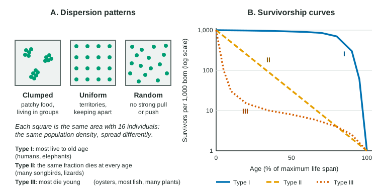
Dispersion is how individuals are spaced within the area (Figure 1, left).
- Clumped: in groups. This is the most common pattern, because resources are patchy (mushrooms on a rotting log, frogs around ponds) and many animals live in social groups (herds, schools).
- Uniform: evenly spaced, because neighbors push each other away. Nesting penguins stay just out of pecking range; some desert shrubs have roots that take water from a wide circle, so a seedling too close to an adult dies.
- Random: no pattern, when individuals neither attract nor repel each other and resources are even, as with some wind-dispersed plants on a uniform field.
Births, deaths and the growth rate
Demography is the study of how births, deaths and movement change a population. Four things change N, the population size: births and immigration (arriving) add individuals; deaths and emigration (leaving) remove them. When migration is small, the formula sheet gives the population growth rate as
dN/dt = B − D
where dN/dt is the change in N per unit time, B is the number of births and D the number of deaths in that time. Dividing by N gives the per capita (per individual) growth rate, which lets you compare populations of different sizes.
Worked example: a deer population. A herd of 400 deer has 120 births and 40 deaths in a year, with no migration.
Step 1. dN/dt = B − D = 120 − 40 = 80 deer per year.
Step 2. Per capita growth rate = 80 ÷ 400 = 0.20 per year: each year the herd grows by a fifth of its size.
Step 3. Per capita birth rate = 120 ÷ 400 = 0.30 per year; per capita death rate = 40 ÷ 400 = 0.10 per year; 0.30 − 0.10 = 0.20, the same answer.
Exponential growth
Under ideal conditions, with plenty of food and space and no crowding, each individual reproduces as fast as its biology allows. The per capita growth rate then reaches its highest value, the intrinsic rate of increase, r_max. Because each individual adds offspring at the same rate however many there are, the number added grows with N. The formula sheet writes this exponential growth as
dN/dt = r_max N
Worked example: a growing culture. A culture of 2,000 yeast cells has r_max = 0.35 per hour. How fast is it growing, and how fast will it grow at 8,000 cells?
Step 1. dN/dt = r_max N = 0.35 × 2,000 = 700 cells per hour.
Step 2. At N = 8,000: dN/dt = 0.35 × 8,000 = 2,800 cells per hour. Four times as many cells, four times as many added per hour.
Step 3. Read the units. r_max is "per hour" (per individual), and dN/dt is "cells per hour". Mixing them up is the most common mistake on this kind of question.
Plot N against time and exponential growth makes a J-shaped curve: flat at first, then ever steeper. A population growing exponentially takes the same time to double whatever its size, so it doubles, doubles again and soon becomes enormous. This is what happened to the pheasants on Protection Island, to rabbits released in Australia, and to bacteria in a fresh broth. It happens only while resources are effectively unlimited: when a population first reaches a new area, or recovers after a crash. Topic 8.4 explains what slows it down.
| If you see | It means |
|---|---|
| The number added each period keeps rising | dN/dt is increasing, as in exponential growth |
| (B − D) ÷ N stays the same each period | The per capita rate is constant: exponential growth |
| The per capita rate falls as N rises | Something limits growth as the population gets crowded (topic 8.4) |
| dN/dt is negative | Deaths (and emigrants) exceed births (and immigrants): the population is shrinking |
Life history: how a species spends its energy
A species' life history is its pattern of reproduction: when it starts, how often, how many offspring, and how much it invests in each. Energy spent on one thing cannot be spent on another, so these traits trade off: an animal can make many cheap offspring or a few expensive ones, not many expensive ones.
Ecologists describe two ends of a range:
| Trait | r-selected (e.g., mice, dandelions, many insects) | K-selected (e.g., elephants, whales, albatrosses) |
|---|---|---|
| Age at first reproduction | Early | Late |
| Offspring per breeding | Many, small | Few, large |
| Parental care | Little or none | Much |
| Life span | Short | Long |
| r_max | High | Low |
| Typical habitat | Unpredictable, often disturbed | Stable, often crowded |
| Usual survivorship | Type III | Type I |
Most species fall somewhere between the two ends, and the r/K labels describe a pattern, not two kinds of species.
A second trade-off is how many times to breed. Semelparity is reproducing once, with an enormous effort, and then dying: Pacific salmon swim upriver, spawn and die; an agave grows for years, sends up one huge flower stalk and dies. Iteroparity is reproducing many times: oak trees produce acorns every year for centuries; most birds and mammals breed in several seasons. Semelparity tends to be favored where adult survival from one breeding season to the next is poor.
Survivorship curves
A life table follows a group born at the same time (a cohort) and records how many are still alive at each age. Plotted as survivors per 1,000 born, on a log scale, against age, it gives a survivorship curve (Figure 1, right). The log scale matters: equal vertical steps mean equal fractions dying (1,000 to 100 and 100 to 10 are both "90% died").
- Type I: high survival until old age, then a steep drop. Large mammals with few, well-cared-for offspring, such as humans and elephants.
- Type II: a straight line on the log scale, meaning the same fraction dies in every age interval. Many songbirds, some lizards.
- Type III: a steep early drop, then a long, slow tail. Oysters, most fish and many plants release huge numbers of eggs or seeds; nearly all die young, and the few that settle in a good place may live long.
Common mistakes
- "Exponential growth adds the same number each year." It adds the same fraction; the numbers added keep rising.
- Confusing r_max (per individual per unit time) with dN/dt (individuals per unit time).
- Reading a log-scale survivorship curve as if it were linear: on a log scale a straight line means a constant fraction dying.
- "Uniform dispersion is the most common." Clumped is; uniform needs something that actively spaces individuals out.
- "r-selected species are less fit." Each life history suits the conditions the species lives in.