Logistic Models — AP® Calculus BC Notes

An exponential model, $\frac{dP}{dt} = kP$ , says the growth rate is proportional to the population, so the population grows without bound. That fits a small population with plenty of food and space, but not a crowded one. A logistic model adds a brake: as the population nears the most the environment can support, its growth slows to zero.

The logistic differential equation

In a logistic model the rate of change is jointly proportional to the population $P$ and to the room left, $K - P$ :

$\frac{dP}{dt} = kP(K - P), \qquad k > 0.$

The same model is often written $\frac{dP}{dt} = rP\left(1 - \frac{P}{K}\right)$ , with $r = kK$ . In both forms, $K$ is the carrying capacity: the positive value of $P$ at which the rate is 0. To read $K$ , set the rate equal to 0 and take the positive solution.

Equation	Carrying capacity	Fastest growth at
$\frac{dP}{dt}$ $= 0.0006P(1200 - P)$	1200	$P = 600$
$\frac{dP}{dt}$ $= 0.04P\left(1 - \frac{P}{2500}\right)$	2500	$P = 1250$
$\frac{dy}{dt} = 2y(7 - y)$	7	$y = 3.5$

Reading the model without solving it

The equilibrium solutions are $P = 0$ and $P = K$ . The sign of $kP(K - P)$ tells what happens from any other starting value:

$0 < P(0) < K$ : the rate is positive, so $P$ increases toward $K$ , never reaching it.
$P(0) > K$ : the factor $K - P$ is negative, so $P$ decreases toward $K$ .
In both cases $\lim_{t \to \infty} P(t) = K$ .

The questions on this topic ask you to interpret the equation: its carrying capacity, its limit, where growth is fastest, what a rate means in context. Solving the equation for a formula is not needed.

Worked example 1. Fish in a lake satisfy $\frac{dP}{dt}$ $= 0.0006P(1200 - P)$ , with $t$ in years and $P(0) = 200$ . Find (a) $\lim_{t \to \infty} P(t)$ , (b) the rate at $t = 0$ , (c) the population when it grows fastest.

(a) The rate is 0 at $P = 1200$ , and $0 < 200 < 1200$ , so $\lim_{t \to \infty} P(t)$ $= 1200$ fish.

(b) $\frac{dP}{dt}$ $= 0.0006(200)(1000)$ $= 120$ fish per year.

Why growth is fastest at half the carrying capacity

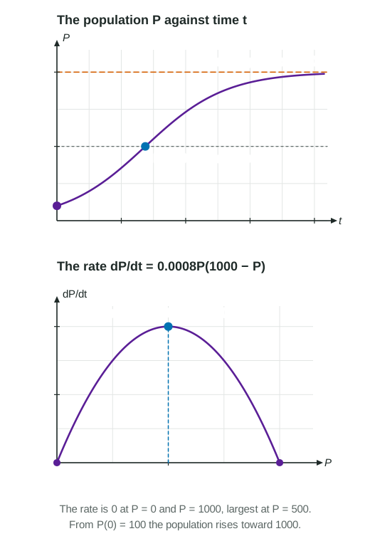
As a function of $P$ , the rate $R(P)$ $= kP(K - P)$ $= kKP - kP^2$ is a downward parabola with zeros at 0 and $K$ . Its derivative $R'(P) = kK - 2kP$ is 0 at $P = \frac{K}{2}$ , where $R$ has its maximum. The figure shows both views: the population against time on the left, the rate against the population on the right.

Left: the population P against time t for dP/dt = 0.0008P(1000 − P) with P(0) = 100. It rises slowly, then steeply, then levels off below the dashed carrying capacity line P = 1000, and is steepest where it crosses P = 500, near t = 2.75, where its concavity changes from up to down. Right: the rate dP/dt against P, a downward parabola that is 0 at P = 0 and P = 1000, with its largest value 200 at P = 500. — **Figure 1.** The population is steepest where the rate parabola peaks, at half the carrying capacity. LevlPrep original diagram.

The same fact gives the concavity of $P(t)$ . By the chain rule,

$\frac{d^2P}{dt^2} = k(K - 2P)\frac{dP}{dt}.$

For a population rising from below $\frac{K}{2}$ , $\frac{dP}{dt} > 0$ , so the graph of $P$ is concave up while $P < \frac{K}{2}$ and concave down while $\frac{K}{2} < P < K$ . The population at $\frac{K}{2}$ is a point of inflection: growth is fastest there.

Worked example 2. In a school of 5000 students, the number $R$ who have heard a rumor satisfies $\frac{dR}{dt}$ $= 0.0002R(5000 - R)$ , with $t$ in hours and $R(0) = 100$ . When is the rumor spreading fastest, and how fast?

Fastest at $R = 2500$ students, half the carrying capacity. The rate then is $0.0002(2500)(2500)$ $= 1250$ students per hour.

In context: when half the school has heard the rumor, it is spreading at 1250 students per hour, faster than at any other time.

Logistic compared with exponential

	Exponential, $\frac{dP}{dt} = kP$	Logistic, $\frac{dP}{dt} = kP(K - P)$
Rate proportional to	$P$	$P$ and $K - P$ , jointly
Long run	grows without bound	approaches $K$
Fastest growth	keeps increasing	at $P = \frac{K}{2}$
Shape of the graph of $P$	concave up	S-shaped: up, then down

For a small population the two models nearly agree, since $K - P \approx K$ and the logistic rate is close to $kKP$ .